Data Assimilation

Cocoa can apply a water level correction produced by data assimilation: a field \(c(x, t)\) in metres that raises (or lowers) the modelled water surface where observations say the model is biased, typically by low-frequency effects the model does not resolve, such as steric anomalies, seasonal mean sea level or remote surge. Cocoa applies the field; computing it from observations (for example by optimal interpolation of observed-minus-modelled anomalies) happens outside the model. The method and an application to Hurricane Matthew are described in [Asher2019]. ADCIRC calls the same feature dynamic water level correction, and Cocoa reproduces it, with the departures listed in Differences from ADCIRC.

Theory

The correction enters the equations as a pseudo atmospheric pressure. The barotropic pressure gradient in the momentum equations, and its counterpart in the GWCE, is taken against the head

\[\eta + \frac{p_a}{\rho_0 g} - \Phi_{\mathrm{tide}} - c,\]

so \(c\) acts exactly like the tidal potential \(\Phi_{\mathrm{tide}}\): in a slowly varying steady state the water surface rises by \(c\). Because it is a pressure, the water has to arrive by flow: a basin behind a narrow inlet fills through the inlet, and its level lags a correction that changes quickly. The correction is also added to the prescribed elevation of open (elevation-specified) boundaries, and to the exterior level of radiation boundaries (codes 30, 32 and 52), which would otherwise radiate a corrected level back out.

With method: pressure_and_mass_adjust (the default, as in ADCIRC), each step’s change \(c^{n+1} - c^n\) is also added directly to the elevation of wet nodes after the GWCE solve, except at open-boundary nodes, which already carry \(c^{n+1}\). The water surface then follows the correction without waiting for flow through inlets, at the cost of mass conservation: the method adds and removes water. The next step’s GWCE time-derivative and advection terms read the solve’s own increment rather than the change in elevation, as ADCIRC does, so the injected water is not replayed as a rise in the following steps. That increment leaves out what the wetting and drying step and the slope limiter change after the solve, so a run with this method and a zero correction is close to, but not identical to, a run without the correction; ADCIRC behaves the same way. With method: pressure only the pressure term acts, mass is conserved, and a zero correction changes nothing.

The figure shows both methods on an idealized ocean, inlet and back basin, with a time-varying correction applied to the basin and a tide at the open boundary. The curves are the basin-mean elevation change against a run without the correction; Cocoa and ADCIRC agree to three decimals. The pressure method lags the correction while it changes and catches up when it is steady; the mass adjust tracks it, overshooting by a few percent while it rises because the pressure term draws water in through the inlet as well.

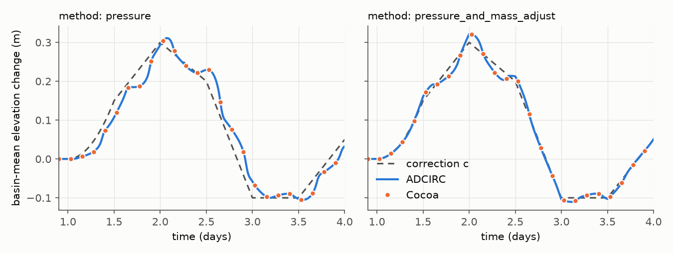
Fig. 8 Basin-mean elevation change caused by the correction (dashed), for the pressure method (left) and the pressure and mass adjust method (right), computed by ADCIRC (line) and Cocoa (dots).

Correction files

The correction is a time series of fields in metres (units of m, meters or metres). Snapshots are interpolated linearly in time; after the last one its values are held, and a file with a single snapshot applies for the whole run. A file with more than one snapshot must span the start of the run, and its time axis must use the standard (proleptic Gregorian) calendar. A value beyond 100 m in either direction stops the run as a broken or mis-scaled file.

format: nodal (the default) is a netCDF file on the mesh’s nodes: a CF time axis, a node dimension equal to the mesh’s node count, and a (time, node) variable (water_level_correction unless variable says otherwise), stored unpacked as float or double. A node holding the variable’s fill value was never written, and stops the run. If the file carries a mesh_id attribute, it must match the mesh.

format: cf_netcdf is a CF file on a regular longitude/latitude grid, read and interpolated bilinearly onto the mesh like CF meteorological forcing: coordinate variables lon, lat and time, data laid out (time, lat, lon), packing and fill values decoded, either latitude order and either longitude convention accepted. A fill value (or NaN) carries no information, so a node whose bilinear stencil touches one takes the average of its other corners, weighted as bilinear interpolation weights them. Nodes outside the grid, and the rare node whose weighted corners are all fill, get no correction. A snapshot that is fill everywhere or holds an infinite value, or a grid that covers no mesh node, stops the run. Startup logs how many nodes lie outside the grid, and a warning reports the number of nodes next to fill whenever it reaches a new high. Rank 0 reads each snapshot grid and sends it to every rank, and each rank interpolates onto its own nodes.

Configuration

The keys are listed in the configuration reference. A forecast cycle that spins up with one correction and hands over to the next on a restart looks like this.

The spin-up run applies the first correction, ramped in after the tide has spun up:

forcing:
  water_level_correction:
    enabled: true
    filename: "correction_cycle_00.nc"
    ramp:
      delay: 10d
      duration: 3d

The forecast run restarts from the spin-up’s checkpoint with a file whose snapshots move from the old correction to the new one, starting at the restart time:

forcing:
  water_level_correction:
    enabled: true
    filename: "correction_cycle_00_to_06.nc"
    ramp:
      delay: 10d
      duration: 3d

Like every ramp (Ramps), the correction’s ramp is measured from the cold start, so the forecast run finds it already complete and the correction continues without a jump. No correction state is checkpointed; every run reads its own file. To bring a correction into a restarted run that had none, start the file’s values at zero at the restart time rather than ramping it: with the mass adjust, whatever the correction has added is part of the checkpointed water level.

Ramp the correction in over hours. A sudden correction acts like a sudden pressure change and can excite spurious waves and a geostrophic current response. On a cold start the water level and the boundaries begin without the correction, so one already in force at the first step arrives as a jump; Cocoa warns when one does.

The applied correction is written as the water_level_correction output variable when it is requested (see Variable Selection).

Differences from ADCIRC

Absolute times

Cocoa’s files carry calendar times. ADCIRC places its first dataset at the start of the run that reads it, so the same file read with a different hotstart time is silently shifted.

Boundary timing

With method: pressure, ADCIRC adds the correction of the previous step to open-boundary elevations; Cocoa adds the current one, as both codes effectively do with the mass adjust.

Radiation boundaries

Cocoa raises a radiation boundary’s exterior level by the correction. ADCIRC leaves it alone; its type 30 boundary holds a corrected level only because its damping term follows the model’s own outflow (see radiation boundaries).

Mass adjust increment

Cocoa does what ADCIRC does here. With the mass adjust, the next step’s time-derivative and advection terms read the solve’s own increment (ADCIRC’s ETAS) instead of the change in elevation, so a zero correction under this method is not exactly a run without one (see Theory).

Ramp

ADCIRC’s ramp is linear between a start and an end offset and can be measured from a hotstart. Cocoa’s is a standard ramp block measured from the cold start: form: linear with a delay is ADCIRC’s ramp, its start the delay and its end the delay plus the duration.

Output timing

ADCIRC’s dynamicWaterlevelCorrection.63 labels each record with its time but writes the previous step’s correction. Cocoa’s water_level_correction is the value applied at the output time.

Gridded input

Cocoa also reads a gridded CF correction file; ADCIRC takes only its nodal ASCII format.