Test Cases

Cocoa includes several test cases that exercise different features and serve both as verification benchmarks but also examples for users to follow along with. Each test case includes a mesh, configuration file, and a plotting script that generates a summary figure.

Channel with Flow

A simple rectangular channel with a specified-flow (type 22) boundary on the upstream (left) end and an open tidal boundary on the downstream (right) end. The top and bottom are land boundaries.

Mesh: 100 x 25 node grid, 10 m uniform depth, ~50 km long channel oriented east-west near the equator.

Forcing: 10,000 m³/s steady inflow on the upstream boundary. The tidal boundary has zero amplitude (still water at the outlet). A 2-day hyperbolic tangent ramp is applied to the flow.

Physics: Manning’s n = 0.025, \(\tau_0\) = 0.005, explicit (lumped) GWCE solver with \(\Delta t\) = 2 s, 3-day simulation.

Expected behavior: Water level rises smoothly during the ramp period and reaches a steady gradient by day 2. The upstream end shows the highest elevation (~0.012 m) with a monotonic decrease toward the downstream open boundary. Velocity is approximately uniform across the channel width.

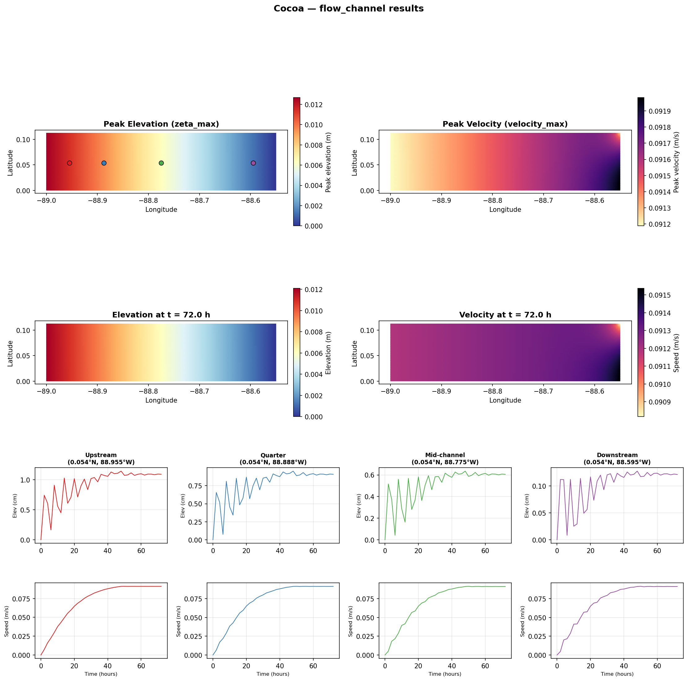
Flow channel (type 22) results showing elevation and velocity maps with probe time series — Fig. 12 Flow channel results. Top row: peak elevation and velocity maps. Middle row: final timestep snapshots. Bottom row: elevation (top) and velocity (bottom) time series at four probe locations along the channel centerline.

Configuration:

output:
  step_interval: 2h

diagnostics:
  screen_interval: 2h

mesh:
  filename: "flow_channel.nc"
  projection:
    type: "EquidistantCylindrical"
    center: [-89.0, 29.0]

simulation:
  start_time: 2026-01-01
  end_time: 2026-01-04
  time_step: 2s

physics:
  manning_n: 0.025
  cf_lower_limit: 0.0025
  tau0: 0.005

forcing:
  ramp:
    enabled: true
    duration: 2d

  tide:
    potential:
      enabled: false
    boundary:
      enabled: true
      constituents:
        - name: M2
          frequency: 1.4051890280e-04
          nodal_factor: 1.0
          equilibrium_arg: 0.0
          boundary_values:    # 26 open boundary nodes, all zero amplitude
            - { amplitude: 0.0, phase: 0.0 }
            # ... (repeated for all 26 nodes)

  flow_boundary:
    enabled: true
    ramp:
      enabled: true
      duration: 2d
    segments:
      - segment_index: 0
        time_series_file: "flow_segment0.yaml"

initial_conditions:
  water_level: 0.0

The flow time series file (flow_segment0.yaml) prescribes a constant 10,000 m³/s inflow:

time_series:
  - { datetime: "2026-01-01 00:00:00", flow: 10000.0 }
  - { datetime: "2026-02-01 00:00:00", flow: 10000.0 }

Note that the tidal boundary is configured with zero amplitude at all nodes — this effectively sets a still-water Dirichlet condition at the downstream open boundary while still requiring the tidal forcing section to be present.

Location: examples/flow_channel/

Channel with Sommerfeld Radiation Boundary and Specified Flow

The same rectangular channel as the type 22 case, but the upstream boundary uses type 32 (specified flow + Sommerfeld radiation) instead of type 22. An M2 tidal signal with 0.005 m amplitude is applied at the downstream open boundary.

Mesh: Identical grid geometry to the flow channel case, but with boundary code 32 on the upstream segment.

Forcing: 10,000 m³/s steady inflow with a prescribed elevation of 0.012 m on the upstream boundary. The downstream boundary has an M2 tidal signal (0.005 m amplitude). Both tidal and flow ramps are 2 days.

Physics: Same as the flow channel case.

Expected behavior: The flow-driven stage ramps up similarly to the type 22 case, but with a superimposed tidal oscillation visible at all probe locations. The radiation term in the \(Q_{\text{force}}\) formulation (see flow boundaries in the GWCE) allows the tidal signal arriving at the upstream boundary to pass through rather than fully reflecting. The upstream probes show the tidal oscillation superimposed on the steady-state flow elevation.

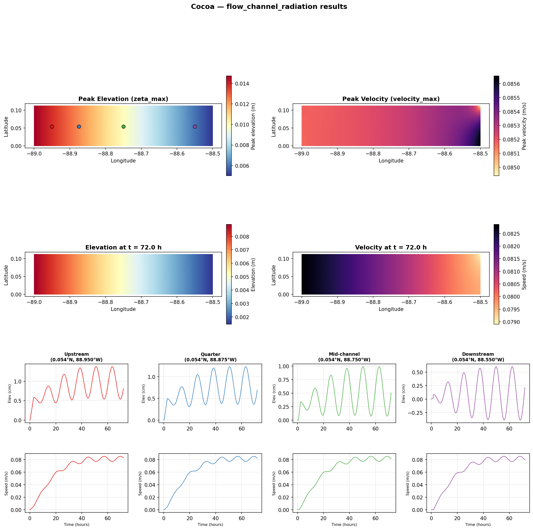
Flow channel with radiation (type 32) results showing tidal oscillation superimposed on flow — Fig. 13 Flow channel with radiation results. The tidal signal from the downstream boundary propagates through the channel and is visible at all probe locations. The upstream probes show tidal oscillation superimposed on the flow-driven stage.

Configuration:

output:
  step_interval: 60

diagnostics:
  screen_interval: 3600

mesh:
  filename: "flow_channel_radiation.nc"
  projection:
    type: "EquidistantCylindrical"
    center: [-89.0, 0.0]

simulation:
  start_time: 2026-01-01
  end_time: 2026-01-04
  time_step: 2s

physics:
  manning_n: 0.025
  cf_lower_limit: 0.0025
  tau0: 0.005

numeric:
  solver: explicit
  gwce_coefficients: [0.0, 1.0, 0.0]

forcing:
  ramp:
    enabled: true
    duration: 2d

  tide:
    potential:
      enabled: false
    boundary:
      enabled: true
      constituents:
        - name: M2
          frequency: 1.4051890280e-04
          nodal_factor: 1.0
          equilibrium_arg: 0.0
          boundary_values:    # 26 open boundary nodes, uniform 0.005 m
            - { amplitude: 0.005, phase: 0.0 }
            # ... (repeated for all 26 nodes)

  flow_boundary:
    enabled: true
    ramp:
      enabled: true
      duration: 2d
    segments:
      - segment_index: 0
        time_series_file: "flow_segment0.yaml"

initial_conditions:
  water_level: 0.0

The flow time series file for this case includes an elevation field, which is required for the radiation term on type 32 boundaries:

time_series:
  - { datetime: "2026-01-01 00:00:00", flow: 10000.0, elevation: 0.012 }
  - { datetime: "2026-02-01 00:00:00", flow: 10000.0, elevation: 0.012 }

Key differences from the type 22 case: the downstream tidal boundary now has a non-zero M2 amplitude (0.005 m), and the flow time series includes a prescribed elevation value used by the Sommerfeld radiation term.

Location: examples/flow_channel_radiation/

Western North Atlantic (WNAT)

A coarse Western North Atlantic domain with tidal and meteorological forcing. This test exercises the full simulation pipeline including tidal boundary conditions, tide potential, meteorological forcing, and wind stress.

Mesh: Coarse unstructured triangular mesh covering the Western North Atlantic, Gulf of Mexico, and Caribbean Sea.

Forcing: M2 tidal constituent on the open ocean boundary with spatially varying amplitude and phase. Tide potential forcing is enabled. CF-NetCDF meteorological forcing provides wind and pressure fields. A 1-day ramp is applied.

Physics: Manning’s n = 0.025, \(\tau_0\) = 0.005, explicit solver with \(\Delta t\) = 20 s, 22-day simulation.

Expected behavior: Tidal oscillations dominate at all probe locations. The Gulf of Mexico probe shows ~1 m tidal range. Wind-driven surge is visible as a low-frequency modulation of the tidal signal. Velocity patterns show strong currents through the Florida Straits and along the shelf break.

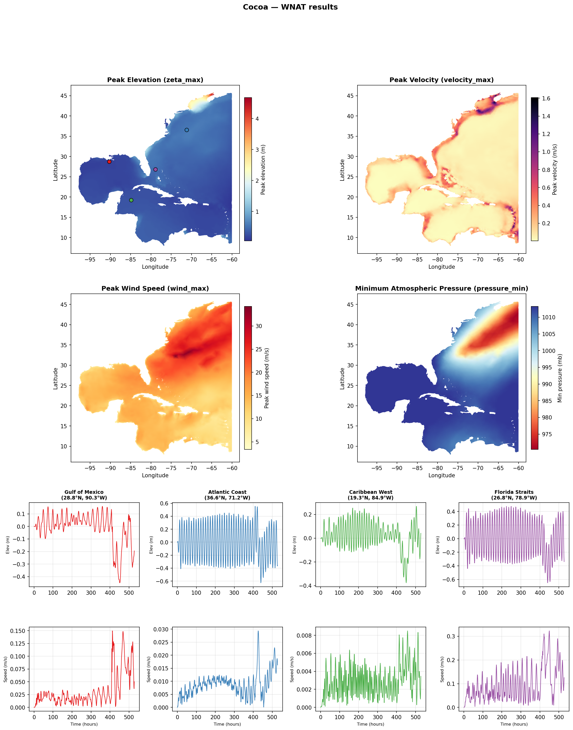
Western North Atlantic results showing tidal and meteorological forcing — Fig. 14 WNAT results. Top row: peak elevation and velocity maps. Middle row: peak wind speed and minimum atmospheric pressure. Bottom row: elevation and velocity time series at four probe locations (Gulf of Mexico, Atlantic Coast, Caribbean West, and Florida Straits).

Configuration (CF-NetCDF meteorological forcing variant):

output:
  step_interval: 180

diagnostics:
  screen_interval: 180
  log_file: log.json

mesh:
  filename: "wnat.nc"
  projection:
    type: "EquidistantCylindrical"
    center: [-76.572766, 23.241697]

simulation:
  start_time: 2026-01-15
  end_time: 2026-02-06
  time_step: 20s

physics:
  manning_n: 0.025
  cf_lower_limit: 0.0010
  tau0: 0.0050000

numeric:
  solver: explicit
  gwce_coefficients: [0.0, 1.0, 0.0]

forcing:
  meteorological:
    enabled: true
    format: cf_netcdf
    filename: "example_met_data/cf_meteo_example.nc"
  ramp:
    enabled: true
    duration: 1d
  tide:
    potential:
      enabled: true
    boundary:
      enabled: true
      constituents:
        - name: M2
          frequency: 1.405189028e-04
          nodal_factor: 0.964086
          equilibrium_arg: 23.057068
          boundary_values:    # 55 open boundary nodes
            - { amplitude: 5.2403779870e-01, phase: 344.168513 }
            - { amplitude: 5.1732976110e-01, phase: 345.153162 }
            # ... (55 nodes with spatially varying amplitude and phase)

This test case also ships with two alternative meteorological forcing configurations: cocoa_config_owi_ascii.yaml (OWI ASCII format) and cocoa_config_owi_netcdf.yaml (OWI NetCDF format). The only difference between the three is the forcing.meteorological section; all other parameters are identical.

Note the use of tide.potential.enabled: true which enables astronomical tide potential body forcing throughout the domain, and the spatially varying tidal boundary values that prescribe M2 amplitudes and phases along the open ocean boundary.

Location: examples/wnat/ (example configurations and met data), test/data/wnat/ (integration test data and reference solutions)

Global Ocean

A global ocean mesh test case that exercises coordinate rotation, Mercator projection, and self-attraction and loading (SAL) tide corrections.

Mesh: Global unstructured triangular mesh with coordinate rotation (pole relocated to avoid the North Pole singularity).

Forcing: Astronomical tide potential with SAL correction. No meteorological forcing. A 5-day ramp is applied.

Physics: Manning’s n from mesh (spatially varying), \(\tau_0\) = 0.0022, Smagorinsky lateral viscosity with coefficient 0.2, implicit (consistent) GWCE solver with \(\Delta t\) = 720 s, 31-day simulation.

Expected behavior: Tidal patterns reproduce the expected global amphidromic system. Large tidal ranges appear in shallow shelf regions (Bay of Fundy, Patagonian shelf, European shelf). Deep ocean amplitudes are modest (~0.5 m). The implicit solver allows the large time step.

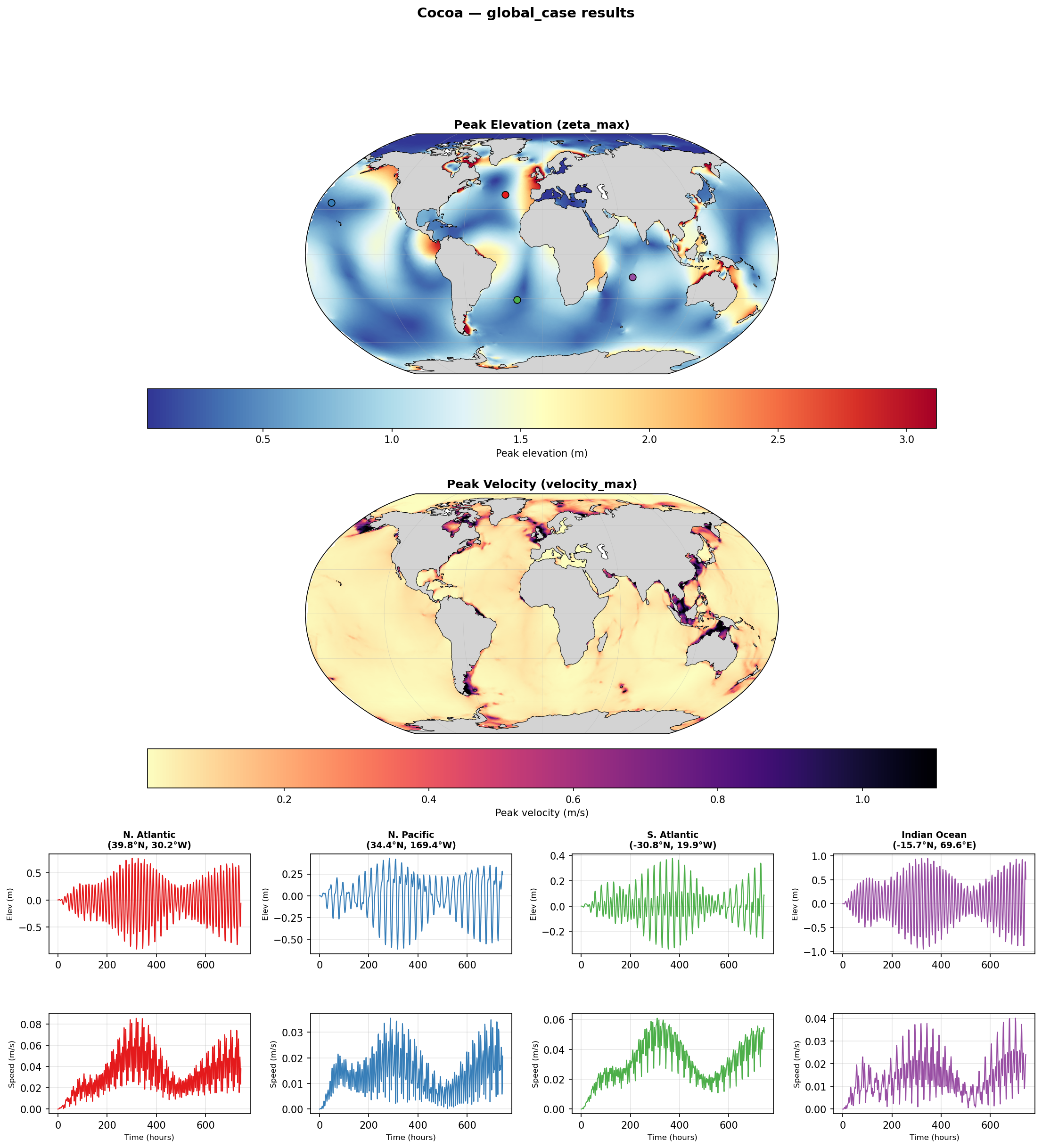
Global ocean results showing tidal amphidromic patterns — Fig. 15 Global ocean results. Top: peak elevation map showing the amphidromic tidal pattern. Middle: peak velocity map. Bottom: elevation and velocity time series at four probe locations (North Atlantic, North Pacific, South Atlantic, Indian Ocean).

Configuration:

output:
  step_interval: 5

diagnostics:
  screen_interval: 60
  log_file: log.json

mesh:
  filename: "global.nc"
  projection:
    type: "Mercator"
    center: [0.0, 45.0]
  rotation:
    enabled: true
    pole_location: [114.16991, 0.77432]

simulation:
  start_time: 2025-01-01
  end_time: 2025-02-01
  time_step: 12m

physics:
  manning_n: "mesh"
  cf_lower_limit: 0.0010
  tau0: 0.0022222
  smagorinsky_coefficient: 0.2
  min_viscosity: 1.0e-6

numeric:
  solver: implicit
  gwce_coefficients: [0.5, 0.5, 0.0]

forcing:
  ramp:
    enabled: true
    duration: 5d
  tide:
    sal:
      enabled: true
    potential:
      enabled: true

initial_conditions:
  water_level: 0.0

This case demonstrates several features unique to global simulations: mesh.rotation relocates the coordinate pole to avoid the North Pole singularity, mesh.projection: Mercator selects the Mercator projection, manning_n: "mesh" reads spatially varying friction from the mesh file, and tide.sal.enabled: true activates the self-attraction and loading correction. The implicit solver (gwce_coefficients: [0.5, 0.5, 0.0]) enables the large 720-second time step. There are no open boundaries in the global mesh, so no tidal boundary forcing is needed.

Location: examples/global_case/