Numerical Methods

Spatial Discretization

Finite Element Mesh

Cocoa uses unstructured meshes of linear (P1) triangles [Hughes2000] [Zienkiewicz2013], optionally mixed with bilinear (Q1) quadrilaterals (Quadrilateral Elements):

• Nodes located at element vertices

• Linear (bilinear) interpolation within elements

• Continuous across element boundaries

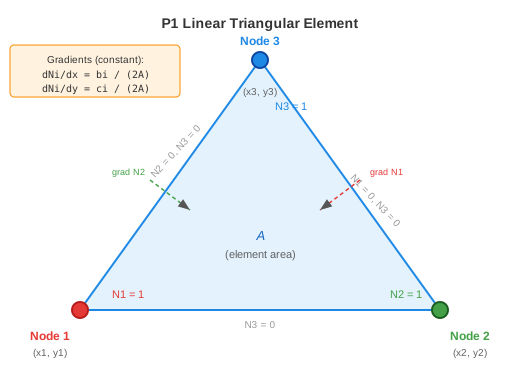
Fig. 44 A P1 linear triangular element. Each shape function Ni equals 1 at its own node and 0 at the other two. Gradients are constant within the element.

Shape Functions

For a triangle with vertices \((x_1, y_1), (x_2, y_2), (x_3, y_3)\), the linear shape functions are:

(25)\[N_i = \frac{1}{2A}(a_i + b_i x + c_i y)\]

where \(A\) is the element area and coefficients are computed from vertex coordinates.

Shape function gradients:

\[\frac{\partial N_i}{\partial x} = \frac{b_i}{2A}, \quad \frac{\partial N_i}{\partial y} = \frac{c_i}{2A}\]

Mass Matrix

Cocoa supports both consistent and lumped mass matrices. The consistent element mass matrix for linear triangular elements is:

(26)\[\begin{split}M^e_{ij} = \int_{\Omega^e} N_i N_j \, d\Omega = \frac{A}{12} \begin{pmatrix} 2 & 1 & 1 \\ 1 & 2 & 1 \\ 1 & 1 & 2 \end{pmatrix}\end{split}\]

The factor \(A/12\) arises from integrating the product of linear shape functions over the element. The off-diagonal entries couple neighboring nodes, providing better accuracy than a lumped formulation.

The lumped mass matrix diagonalizes the mass matrix by row-summing:

\[M^e_{ii} = \frac{A}{3}, \quad M^e_{ij} = 0 \text{ for } i \neq j\]

The lumped formulation enables an explicit direct solve (no iterative solver needed) at the cost of some spatial accuracy. The GWCE-specific mass matrix formulation including \(\tau_0\) weighting is given in Equation (12). See Configuration for solver selection.

Quadrilateral Elements

Cocoa also runs on bilinear (Q1) quadrilaterals [Hughes2000] [Zienkiewicz2013], and on hybrid meshes mixing triangles and quadrilaterals in a single partition. Everything below is computed once per element at startup and cross-referenced to the code that implements it. Both element types share that code: the reference element – cubature points and weights, basis values and reference gradients – comes from Intrepid2 [Bochev2012] through geometry/ReferenceElement.{hpp,cpp}, the element evaluation itself is geometry/ElementGeometry.hpp (one body, run by the host table fill and by the device recompute of a rotated mesh alike), and the uploaded device storage is geometry/ElementTables.hpp. Only ReferenceElement.cpp includes Intrepid2; the tags take their topology keys from Shards’ own header, and everything past the reference element sees plain fixed-size arrays.

Corners \(p_i = (x_i, y_i)\), \(i = 0..3\), are stored counter-clockwise with cyclic indices (mod 4) in the same projected coordinates the triangle uses.

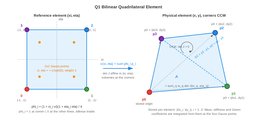
Fig. 45 A Q1 bilinear quadrilateral. Left: the reference square, corners at \((\xi_i, \eta_i) = (\pm 1, \pm 1)\) numbered counter-clockwise from \((-1, -1)\), with the four Gauss points at \(\pm 1/\sqrt{3}\). Right: the physical element the bilinear map produces, its corners stored as offsets from corner 0, the chord \(p_1 p_3\) whose components are corner 2’s Green coefficients, and the counter-clockwise orientation that keeps \(\det J\) positive.

Green coefficients. The quadrilateral analogue of ADCIRC’s FDX/FDY is

(27)\[b_i = y_{i+1} - y_{i-1}, \qquad a_i = x_{i-1} - x_{i+1}\]

so that \(b_i/(2A)\) and \(a_i/(2A)\) are the exact area-averaged \(x\)- and \(y\)-derivatives of basis function \(i\), the same role the triangle’s \(b_i = y_j - y_k\), \(a_i = x_k - x_j\) play there. At three vertices Equation (27) reduces identically to the triangle formula: Geometry::green_coefficients is templated on the element-type tag so a test can pin that reduction bit-for-bit against the classical triangle spelling, and a second test pins both instantiations against the basis gradients Intrepid2 integrates. The construction identities checked at \(10^{-12}\) on random convex quadrilaterals are \(\sum_i b_i = \sum_i a_i = 0\), \(\sum_i b_i x_i = \sum_i a_i y_i = 2A\), \(\sum_i b_i y_i = \sum_i a_i x_i = 0\), and for any field linear in \((x, y)\), \(\sum_i f_i b_i / (2A)\) recovers \(\partial f/ \partial x\) exactly (and the \(a_i\) analogue for \(y\)) – so every ADCIRC term of the form “element-averaged forcing times the gradient of a test function” carries over from the triangle unchanged, with \(N = 4\) and the nodal mean \(\tfrac{1}{4}\sum_i\) in place of the triangle’s \(\tfrac{1}{3}\sum_i\).

Bilinear reference map. With reference coordinates \((\xi, \eta) \in [-1, 1]^2\) and corner signs \((\xi_i, \eta_i) = (-1,-1), (1,-1), (1,1), (-1,1)\):

\[\phi_i = \tfrac{1}{4}(1 + \xi_i \xi)(1 + \eta_i \eta), \qquad \frac{\partial \phi_i}{\partial \xi} = \tfrac{1}{4}\xi_i(1 + \eta_i \eta), \qquad \frac{\partial \phi_i}{\partial \eta} = \tfrac{1}{4}\eta_i(1 + \xi_i \xi)\]

\[\begin{split}J = \begin{bmatrix} \partial x/\partial\xi & \partial x/\partial\eta \\ \partial y/\partial\xi & \partial y/\partial\eta \end{bmatrix}, \qquad |J| = \frac{\partial x}{\partial\xi}\frac{\partial y}{\partial\eta} - \frac{\partial x}{\partial\eta}\frac{\partial y}{\partial\xi}\end{split}\]

with \(\partial x/\partial\xi = \sum_i x_i\, \partial\phi_i/\partial\xi\) and so on, and \(|J| > 0\) everywhere on a convex, counter-clockwise quadrilateral. The physical gradients follow from the standard isoparametric inverse-Jacobian relations.

2x2 Gauss integration and why full, not reduced. The element operators have no closed form on a general straight-sided quadrilateral (unlike the triangle’s area-only formulas), so they are integrated numerically, once, at startup:

(28)\[\begin{split}\begin{aligned} M_{ij} &= \sum_q \phi_i(q)\,\phi_j(q)\,|J(q)|, \\ K^{xx}_{ij} &= \sum_q \frac{\partial \phi_i}{\partial x}(q)\, \frac{\partial \phi_j}{\partial x}(q)\,|J(q)|, \\ K^{yy}_{ij} &= \sum_q \frac{\partial \phi_i}{\partial y}(q)\, \frac{\partial \phi_j}{\partial y}(q)\,|J(q)| \end{aligned}\end{split}\]

at the four points \((\pm 1/\sqrt{3}, \pm 1/\sqrt{3})\) with unit weights. The mass integrand is bilinear on a straight-sided quadrilateral, so 2x2 Gauss is exact for \(M\) and for every identity the tests check; \(K^{xx}\) and \(K^{yy}\) are exact on parallelograms and a converged approximation otherwise. One-point (reduced) integration at the centroid is not used: a bilinear quadrilateral under one-point quadrature has a spurious zero-energy deformation mode (the Q1 “hourglass” mode, a strain field that vanishes at the centroid but not elsewhere), and suppressing it needs an hourglass-control term [Flanagan1981] with no counterpart in the triangle path or in the GWCE gravity-wave operator. Full integration avoids the problem at the cost of four cubature points per operator entry.

Construction-level identities checked at \(10^{-12}\) on random convex quadrilaterals: \(\sum_{ij} M_{ij} = A\); \(M\) symmetric with every entry positive; the row sums of \(K^{xx}\) and \(K^{yy}\) are zero (the constant, or rigid, mode carries no gravity-wave energy); \(K^{xx}, K^{yy}\) symmetric positive semi-definite; \((K^{xx} x)_i = b_i/2\) and \((K^{yy} y)_i = a_i/2\) exactly (the integrand is polynomial); \((K^{xx} y)_i = (K^{yy} x)_i = 0\). On a rectangle \(a \times b\) the operators reduce to the closed forms

\[\begin{split}\begin{aligned} M &= \frac{ab}{36}\begin{pmatrix}4&2&1&2\\2&4&2&1\\1&2&4&2\\2&1&2&4\end{pmatrix}, \\ K^{xx} &= \frac{b}{6a}\begin{pmatrix}2&-2&-1&1\\-2&2&1&-1\\-1&1&2&-2\\1&-1&-2&2\end{pmatrix}, \\ K^{yy} &= \frac{a}{6b}\begin{pmatrix}2&1&-1&-2\\1&2&-2&-1\\-1&-2&2&1\\-2&-1&1&2\end{pmatrix} \end{aligned}\end{split}\]

checked at \(10^{-14}\), invariant under rotation and translation of the rectangle.

Storage: the corners, not the operators. Nothing about a quadrilateral’s operators is stored. The table keeps the element’s three corner offsets relative to corner 0 (6 doubles, 48 bytes), and each kernel integrates from them what its thread owns. A thread that owns one matrix row integrates that row (Geometry::element_operator_row): 4 entries each of \(M\), \(K^{xx}\) and \(K^{yy}\), 12 doubles out of 6 loads. A thread that owns a whole element – the GWCE right-hand side, the lumped diagonal, the lumping weights of the nodal accumulators – integrates the whole element once (Geometry::element_operators), because integrating a row at a time would repeat the Jacobian and the physical gradients once per vertex; measured, that cost the right-hand side 34% against integrating the element once. The three packed symmetric operators and the lumped rows that were stored instead – 34 doubles, 272 bytes per quadrilateral – were the largest dependent load chain left in the assembly kernels once the CSR row search was removed, and the arithmetic that replaces them (about 400 flops per element) is not what those kernels are short of. The packed symmetric layout – the 10 upper-triangle entries of a \(4\times4\) operator in the row-major order \((0,0), (0,1), (0,2), (0,3), (1,1), (1,2), (1,3), (2,2), (2,3), (3,3)\), Geometry::packed_index – is how the whole-element form returns them.

The recompute is bit-identical to the storage it replaces, not equal to within a tolerance: a row accumulates over the same cubature points in the same order out of the same Jacobian, and IEEE multiplication commutes exactly, so the entry below the diagonal that the packed storage held as \(\phi_j\phi_i\) is the same double as the \(\phi_i\phi_j\) the row forms. A unit test pins every entry of every row against the whole element’s operators with an exact comparison.

The identity holds wherever the compiler does not fuse a multiply-add. A fused term is rounded once where a separate multiply and add round twice, and which terms a compiler fuses depends on what it inlined and vectorized around them, so two loop shapes over the same arithmetic can differ in the last bit on any FMA target: a GPU build, where the operators are formed by the device compiler inside the assembly kernels, and equally an FMA host. What holds everywhere is the bound the mechanism predicts, one saved rounding per fused term. The bit-identity gate rests on a single toolchain generating and comparing its own integration references.

The same operators serve all three GWCE time levels: the LHS gravity-wave term (coefficient \(a_{00}\)) and both RHS gradient terms (\(b_{00}\), \(c_{00}\)) integrate the identical \(K^{xx}\), \(K^{yy}\) for a given quadrilateral – there is no separate operator per time level, unlike the mass-matrix pattern which does depend on solver type (Lumped vs Consistent Mass Matrix).

Lumped mass and nodal averages. The lumped row \(ML_i = \sum_j M_{ij} = \int_\Omega \phi_i \, d\Omega\) (exactly \(A/4\) on a parallelogram) plays the quadrilateral’s role in the lumped solver and in every “area times value” nodal accumulator (the lumping convention). The quadrilateral element average of a nodal field is the plain nodal mean \(\tfrac{1}{4}\sum_i f_i\), the triangle’s \(\tfrac{1}{3}\sum_i f_i\) with \(N = 4\).

Conditioning: corners relative to corner 0. Absolute projected coordinates run to \(10^6\)-\(10^7\) m while an element edge is \(O(10^2)\) m; the shoelace area and the Gauss sums above difference pairs of such coordinates, which loses about six decimal digits if done on the raw absolute values (measured 2e-6 relative error in area at \(10^6\) m production offsets, degrading the identities above from \(10^{-12}\) to \(10^{-10}\)). Every sum that would otherwise difference two absolute coordinates instead translates the four corners so corner 0 becomes exactly \((0,0)\) first (Geometry::corners_relative_to_first); every other corner is then one subtraction of two nearby doubles, which is exact. Area and both element operators are translation-invariant, so this changes nothing mathematically. The Green coefficients (Equation (27)) need no such translation: each one is already a single subtraction of two nearby coordinates.

The wet/dry corner rules a quadrilateral needs beyond the geometry above – its dry corners are not always edge neighbors of its wet ones, unlike a triangle – are Quadrilateral Rules (W1, DE1) in Wetting and Drying.

Temporal Discretization

Time Integration Scheme

Cocoa uses a three-level scheme for the GWCE:

\[\frac{\partial^2 \zeta}{\partial t^2} \approx \frac{\zeta^{n+1} - 2\zeta^n + \zeta^{n-1}}{\Delta t^2}\]

\[\frac{\partial \zeta}{\partial t} \approx \frac{\zeta^{n+1} - \zeta^{n-1}}{2\Delta t}\]

This provides second-order accuracy in time.

Momentum equations use a semi-implicit Crank-Nicolson scheme for the pressure gradient and bottom friction terms, with explicit treatment of advection and lateral stress.

Linear Solver

Assembly Pattern: Scatter-to-Gather

Every assembly in the CG solver – the GWCE right-hand side, the lumped diagonal, the momentum right-hand sides and the consistent GWCE matrix – is an element-parallel scatter: a thread evaluates one wet element’s rows and adds them to the node-indexed target with Kokkos::atomic_add, three rows for a triangle and four for a quadrilateral. Where the target is the sparse matrix the two element types reach it differently. The triangle path hands each row to sumIntoValues, which finds every column by a search along the CSR row; the quadrilateral path resolves the column position of each of its sixteen entries once at startup, so a thread per (element, row) adds straight into the value array. Elements that touch ghost nodes add into the rank’s overlap rows; one export after the scatter sums those rows into their owners (sum_into_owned for vectors, FECrsMatrix::endAssembly for the matrix), and the per-row fix-ups – boundary conditions, dry rows – run on owned rows only, after the export.

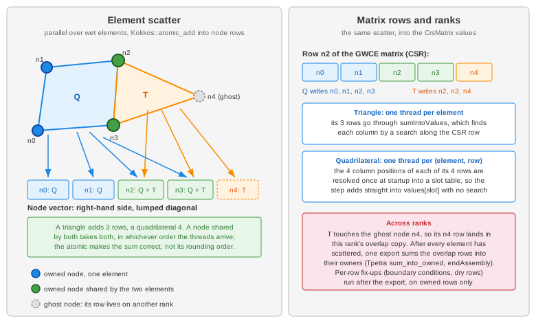
Fig. 46 A quadrilateral and a triangle that share an edge scatter into the same node rows: the two shared nodes receive both elements’ contributions, the ghost node’s row is summed into its owning rank by the export. The matrix panel shows the one place the element types differ, the row search of the triangle path against the precomputed slot of the quadrilateral path.

System Assembly

The GWCE produces a sparse linear system:

(29)\[\mathbf{A} \boldsymbol{\zeta}^{n+1} = \mathbf{b}\]

The matrix \(\mathbf{A}\) has the sparsity pattern of the mesh connectivity (see the GWCE discretization in Equation (12) and (13)).

Iterative Solver

Cocoa uses the Conjugate Gradient (CG) method via the Belos solver package from Trilinos [Heroux2005] [Bavier2012]:

\[\begin{split}&\mathbf{r}_0 = \mathbf{b} - \mathbf{A}\mathbf{x}_0 \\ &\mathbf{p}_0 = \mathbf{r}_0 \\ &\text{for } k = 0, 1, 2, \ldots \\ &\quad \alpha_k = (\mathbf{r}_k, \mathbf{r}_k) / (\mathbf{p}_k, \mathbf{A}\mathbf{p}_k) \\ &\quad \mathbf{x}_{k+1} = \mathbf{x}_k + \alpha_k \mathbf{p}_k \\ &\quad \mathbf{r}_{k+1} = \mathbf{r}_k - \alpha_k \mathbf{A}\mathbf{p}_k \\ &\quad \beta_k = (\mathbf{r}_{k+1}, \mathbf{r}_{k+1}) / (\mathbf{r}_k, \mathbf{r}_k) \\ &\quad \mathbf{p}_{k+1} = \mathbf{r}_{k+1} + \beta_k \mathbf{p}_k\end{split}\]

Preconditioning

Jacobi preconditioning is applied:

\[\mathbf{M}^{-1} = \text{diag}(\mathbf{A})^{-1}\]

This improves convergence while maintaining GPU efficiency.

Convergence Criteria

The solver terminates when the scaled residual norm satisfies the tolerance. By default, Cocoa scales the residual by the initial residual norm (NormOfInitialResidual):

\[\frac{\|\mathbf{r}_k\|}{\|\mathbf{r}_0\|} < \epsilon\]

with default tolerance \(\epsilon = 10^{-5}\).

The convergence scaling is selectable; the three available options are:

• NormOfInitialResidual (default): \(\|\mathbf{r}_k\| / \|\mathbf{r}_0\| < \epsilon\)

• NormOfPrecInitRes: \(\|\mathbf{M}^{-1}\mathbf{r}_k\| / \|\mathbf{M}^{-1}\mathbf{r}_0\| < \epsilon\)

• None: \(\|\mathbf{r}_k\| < \epsilon\) (absolute tolerance)

Numerical Stability

CFL Condition

For a stable explicit time step, the Courant-Friedrichs-Lewy (CFL) condition provides useful guidance for choosing \(\Delta t\):

(30)\[\Delta t \lesssim C \cdot \min_e \frac{h_e}{\sqrt{gH_e}}\]

where \(h_e\) is the element size and \(C \approx 0.5\) is the Courant number. This is descriptive guidance, not an enforced constraint: Cocoa only validates that the configured time step is positive and does not compute a CFL-limited step internally. The user is responsible for selecting a stable \(\Delta t\).

Numerical Diffusion

Explicit advection schemes introduce numerical diffusion. This is partially offset by the GWCE formulation.

Floating-Point Precision

Cocoa performs all arithmetic in double precision (FP64). Both the lumped (explicit) and consistent (implicit) GWCE solvers, the momentum solver, and all reductions accumulate in double; the consistent mass matrix in particular requires it to avoid overflow in the iterative solve.

Mixed-precision storage. To cut memory traffic without changing the numerics, a subset of bandwidth-sensitive fields is stored as single precision (float) and promoted to double the moment it is read into a kernel:

• the prognostic velocity and flux fields,

• the bottom-friction and lateral-stress tensors,

• a subset of static mesh geometry (element areas, scale factors, Coriolis, tan_phi, and the element-averaged bathymetry), the slope-limiter coefficients, and nodal attributes.

Bathymetry itself and the spatial gradient coefficients (the a and b shape-function derivative arrays) remain double precision, as do water-surface elevation, the GWCE/momentum right-hand sides, the assembled system matrices, and all accumulators.

The float/double conversions are confined to a single sanctioned boundary at the gather/scatter step (Cocoa::Types::promote reads float storage up to double; Cocoa::Types::narrow writes a double result back to float). promote is an exact no-op when the field is double-stored, so read sites are written uniformly regardless of a field’s storage precision; narrow always truncates and is used only at float storage boundaries. Because the working arithmetic is unchanged, the only numerical effect is the ~1e-7 relative round-off incurred when a float-stored field is written and later re-read.

Performance considerations. This scheme targets GPU architectures, where memory bandwidth — not double-precision throughput — is usually the limiting factor; storing the heavily-streamed fields as float reduces the bytes moved per timestep. CPU architectures see little benefit, as they already hide the extra bandwidth of full double-precision storage, but they are unaffected because compute precision is identical in both cases.