Generalized Wave Continuity Equation (GWCE)

The Generalized Wave Continuity Equation (GWCE) is a reformulation of the continuity equation that provides improved numerical stability for finite element discretizations [Luettich1992]. Cocoa implements the GWCE formulation as described in the ADCIRC theory documentation, following the spherical coordinate formulation of [Kolar1994].

Motivation

The primitive continuity equation (see (6)):

(10)\[\frac{\partial \zeta}{\partial t} + \nabla \cdot (\mathbf{Q}) = 0\]

where \(\mathbf{Q} = H\mathbf{U}\) is the flux vector, poses numerical challenges when solved with standard Galerkin finite elements on the same mesh as the momentum equations [Dawson2006]. The GWCE addresses these issues by incorporating wave-like behavior through time differentiation.

GWCE Derivation

The GWCE is derived by:

1. Differentiating the continuity equation with respect to time

2. Substituting the momentum equations for \(\partial \mathbf{Q}/\partial t\)

3. Adding a weighted form of the original continuity equation

This yields the full GWCE:

(11)\[\frac{\partial^2 \zeta}{\partial t^2} + \tau_0 \frac{\partial \zeta}{\partial t} - \nabla \cdot \left[ gH \nabla\zeta + \mathbf{J} \right] - \tau_0 \nabla \cdot \mathbf{Q} = 0\]

where \(\mathbf{J} = (J_x, J_y)\) contains the momentum equation terms.

Momentum Terms (J Vector)

The \(\mathbf{J}\) vector in Equation (11) includes:

Coriolis with Spherical Correction:

\[J_x^{cor} = f_{eff} Q_y, \quad J_y^{cor} = -f_{eff} Q_x\]

where \(f_{eff} = f + \frac{U \tan\phi}{R}\) includes the spherical metric correction.

Bottom Friction (TKM Tensor):

\[J_x^{fric} = -(\tau_{xx} Q_x + \tau_{xy} Q_y), \quad J_y^{fric} = -(\tau_{xy} Q_x + \tau_{yy} Q_y)\]

Tau0 Weighting:

\[J_x^{\tau_0} = \tau_0 Q_x, \quad J_y^{\tau_0} = \tau_0 Q_y\]

Wind Stress:

\[J_x^{wind} = \frac{R_{met}}{3\rho_0} \sum_{i=1}^{3} f_{w,i} \, \tau_{sx,i}, \quad J_y^{wind} = \frac{R_{met}}{3\rho_0} \sum_{i=1}^{3} f_{w,i} \, \tau_{sy,i}\]

where \(\boldsymbol{\tau}_s\) is computed from the Garratt drag law and \(f_{w,i}\) is the depth-dependent wind stress limiter evaluated per node. See Meteorological Forcing for the complete formulation.

Atmospheric Pressure Gradient:

\[J_x^{atm} = -\frac{\alpha_L \bar{H}}{\rho_0} \frac{\partial p_s}{\partial x}, \quad J_y^{atm} = -\frac{\alpha_L \bar{H}}{\rho_0} \frac{\partial p_s}{\partial y}\]

See Meteorological Forcing for discretization and pressure ramping.

Lateral Stress Divergence:

\[J_x^{ls} = \frac{\partial \sigma_{xx}}{\partial x} + \frac{\partial \sigma_{xy}}{\partial y} - \frac{\tan\phi}{R}(\sigma_{xy} + \sigma_{yx})\]

Advection (Non-Conservative Form):

\[J_x^{adv} = -\left(Q_x \frac{\partial U}{\partial x} + Q_y \frac{\partial U}{\partial y}\right)\]

Discretized J Vector Assembly

The continuous J vector terms above are discretized using linear triangular finite elements. For an element with nodes \((1, 2, 3)\), area \(A_e\), and shape function derivatives \(\partial N_i/\partial x\), the following discretized forms are computed.

Shape Function Derivative Products:

The finite element derivatives are stored as \(FDX_i = 2 A_e \frac{\partial N_i}{\partial x}\) and \(FDY_i = 2 A_e \frac{\partial N_i}{\partial y}\). Element gradients are computed as:

\[\frac{\partial \phi}{\partial x} = \frac{1}{2A_e} \, \sum_{i=1}^{3} \phi_i \cdot FDX_i\]

Coriolis (Discretized):

\[J_x^{cor,e} = \bar{f}_{eff} \cdot \bar{Q}_y, \quad J_y^{cor,e} = -\bar{f}_{eff} \cdot \bar{Q}_x\]

where \(\bar{Q}_x = \frac{1}{3} \, \sum_{i=1}^{3} Q_{x,i}\) is the element-averaged flux, and \(\bar{f}_{eff} = \bar{f} + \bar{\tan\phi} \cdot \bar{U}\) includes the spherical metric correction.

Bottom Friction (Discretized):

\[J_x^{fric,e} = -\frac{1}{3} \, \sum_{i=1}^{3} \bigl(\tau_{xx,i} \, Q_{x,i} + \tau_{xy,i} \, Q_{y,i}\bigr)\]

The TKM tensor values are stored at nodes and averaged over the element.

Tau0 Weighting (Discretized):

\[J_x^{\tau_0,e} = \frac{1}{3} \, \sum_{i=1}^{3} \tau_{0,i} Q_{x,i}\]

Advection (Discretized):

The advection term has spatial and temporal components:

Spatial term:

\[\begin{split}\begin{split} J_x^{adv,spatial} &= -\bar{Q}_x \frac{\partial U}{\partial x} - \bar{Q}_y \frac{\partial U}{\partial y} \\ &= -\frac{1}{2A_e}\left( \bar{Q}_x \sum_i U_i \cdot FDX_i + \bar{Q}_y \sum_i U_i \cdot FDY_i \right) \end{split}\end{split}\]

Temporal term (convective acceleration):

\[J_x^{adv,temporal} = \bar{U} \cdot \frac{\bar{\zeta}^n - \bar{\zeta}^{n-1}}{\Delta t}\]

This term accounts for the time derivative of momentum due to changing water levels.

Lateral Stress (Discretized):

\[\begin{split}\begin{split} J_x^{ls,e} = \frac{1}{2A_e}\bigl( &\sum_i \sigma_{xx,i} \cdot FDX_i + \sum_i \sigma_{xy,i} \cdot FDY_i\bigr) \\ &- \bar{\tan\phi} \cdot (\bar{\sigma}_{xy} + \bar{\sigma}_{yx}) \end{split}\end{split}\]

Element Contribution to Global RHS:

The total J vector contribution from each element is distributed to its three nodes and accumulated into the global RHS vector using atomic operations:

\[RHS_i \mathrel{+}= \frac{1}{2} \left( J_x^e \cdot FDX_i + J_y^e \cdot FDY_i \right)\]

Since \(FDX_i = 2 A_e \frac{\partial N_i}{\partial x}\), this is equivalent to:

\[RHS_i \mathrel{+}= A_e \left( J_x^e \frac{\partial N_i}{\partial x} + J_y^e \frac{\partial N_i}{\partial y} \right)\]

On quadrilaterals. Every J-vector term above generalizes to a quadrilateral by substituting \(N = 4\), the quadrilateral Green coefficients \(b_i, a_i\) (Quadrilateral Elements) for \(FDX_i, FDY_i\), and the quadrilateral nodal mean \(\tfrac{1}{4}\sum_{i=1}^{4}\) for the triangle’s \(\tfrac{1}{3}\sum_{i=1}^{3}\) everywhere an element average such as \(\bar{Q}_x\), \(\bar{U}\), or the TKM/tau0 averages appears – Coriolis, bottom friction, tau0 weighting, advection, and lateral stress alike. Both element types are assembled by the one tag-templated body in continuity/GwceVectorAssemblyKernels.hpp; the quadrilateral launch runs into the same nodal RHS accumulators immediately after the triangle one, on quadrilateral-bearing meshes only.

GWCE Parameter (\(\tau_0\))

The GWCE parameter \(\tau_0\) is a positive weighting factor that controls the relative contribution of the primitive continuity equation versus the wave equation form. It provides numerical stability by damping spurious oscillations.

• Larger \(\tau_0\): Stronger weighting toward primitive continuity equation

• Smaller \(\tau_0\): Behavior closer to pure wave equation

• Typical values: 0.001 to 0.05

Cocoa Implementation:

Cocoa supports spatially varying \(\tau_0\) via mesh nodal attributes (primitive_weighting_in_continuity_equation), allowing different values in different regions of the domain. The value must always be positive. Set tau0: mesh in the YAML configuration to use spatially-varying values.

Coordinate Systems

Cocoa supports multiple cylindrical map projections for spherical coordinates. The default is the equidistant cylindrical (CPP) projection, corresponding to ADCIRC’s ICS=21 setting. See Coordinate Systems for complete details on available projections.

Key points for GWCE assembly:

• The stiffness matrix uses projection scale factors \(C_x\) and \(C_y\) to correct gradient products (see Equidistant Cylindrical (Default))

• Mass matrix terms are weighted by \(\cos\phi\) at each node to account for the spherical area element

• Lateral stress terms include a \(\tan\phi/R\) correction for spherical geometry:

\[J_x^{ls} = \frac{\partial \sigma_{xx}}{\partial x} + \frac{\partial \sigma_{xy}}{\partial y} - \frac{\tan\phi}{R}(\sigma_{xy} + \sigma_{yx})\]

Finite Element Discretization

Cocoa uses linear triangular elements with Galerkin weighting. The weak form integrates by parts to yield:

Mass Matrix Term:

For the temporal terms, the elemental mass matrix contribution is:

(12)\[\begin{split}M_{ij}^e = \frac{A_e}{12 \Delta t} \left( \frac{1}{\Delta t} + \frac{\tau_0}{2} \right) \cdot S_i \cdot \begin{cases} \text{OnDiag} & i = j \\ \text{OffDiag} & i \neq j \end{cases}\end{split}\]

where \(S_i = \cos\phi_i\) is the nodal scale factor accounting for spherical area. The diagonal and off-diagonal coefficients depend on the solver type (see Lumped vs Consistent Mass Matrix).

This factor is computed in gwce_mass_matrix_factor() using the constant MASS_MATRIX_FACTOR = 1/12.

Stiffness Matrix Term:

The stiffness matrix discretizes the \(\nabla \cdot (gH\nabla\zeta)\) term:

(13)\[K_{ij}^e = \frac{\alpha_L \cdot g \cdot a_{00} \cdot \bar{H}}{4 A_e} \left( C_x \frac{\partial N_i}{\partial x} \frac{\partial N_j}{\partial x} + C_y \frac{\partial N_i}{\partial y} \frac{\partial N_j}{\partial y} \right)\]

where:

• \(\alpha_L\) is the slope limiter from wet/dry (reduces gradients in shallow water)

• \(a_{00}\) is the temporal integration coefficient for \(\zeta^{n+1}\)

• \(\bar{H}\) is the element-averaged total water depth

The scale factors \(C_x\) and \(C_y\) account for spherical geometry in the CPP projection. For ICS=21:

\[C_x = \frac{1}{S_x^2} = \frac{\cos^2\phi}{\cos^2\phi_0}, \quad C_y = 1\]

These factors arise because the stiffness matrix involves products of derivatives. Since x-derivatives are scaled by \(S_x = \cos\phi_0/\cos\phi\), the product \((\partial/\partial x)^2\) gains a factor of \(S_x^2\), which is then divided out to recover the correct physical gradient.

On quadrilaterals. A quadrilateral has no closed-form mass or stiffness matrix analogous to \(A_e/12\) and \(b_i b_j/(4A_e)\): both are integrated by 2x2 Gauss quadrature from the element’s corners, wherever they are needed (Quadrilateral Elements). The same \(K^{xx}_{ij}\), \(K^{yy}_{ij}\) serve Equation (13)’s \(a_{00}\) LHS term and the \(b_{00}\)/\(c_{00}\) RHS gradient terms below – there is one operator per quadrilateral, not one per time level – and the scale factors \(C_x\), \(C_y\) apply identically. The consistent and lumped assemblies insert \(M_{ij} S_j\) and \(\alpha_L g a_{00} \bar{H} (C_x K^{xx}_{ij} + C_y K^{yy}_{ij})\) into the same global system the triangle assembly builds, mirroring Equations (12) and (13) term for term with the quadrilateral’s integrated operators in place of the triangle’s closed forms.

The lumping convention. Every nodal accumulator that a scatter later divides by – active_element_area, total_element_area, and any other “area times value” sum – weights an element’s contribution to a node by \(3 \times \int_{\Omega^e}\phi_i\,d\Omega\) (the constant Geometry::lumped_area_weight times \(\int\phi_i\), both applied by Geometry::element_lumped_area_weights), not by the element’s own area. On a triangle \(\int \phi_i\,d\Omega = A_e/3\) at every vertex, so this is exactly the triangle’s area – the quantity the triangle kernels have always scattered. On a quadrilateral \(\int\phi_i\,d\Omega = ML_i\) (the lumped mass row, about \(A_e/4\) and unequal between corners on anything but a parallelogram), so its weight is \(3\,ML_i\), not its area – using the area instead would over-weight a quadrilateral by \(4/3\) against a triangle sharing the node. The lateral-stress divergence factor of 1.5 (momentum RHS, Momentum Equations) is unaffected and stays the same constant for both element types; only the area-weighted accumulators carry the per-type factor. The triangle path is unchanged (its weight is its area), and the quadrilateral path integrates exactly.

Time Discretization

Cocoa uses a three-level scheme with coefficients \(a_{00}, b_{00}, c_{00}\):

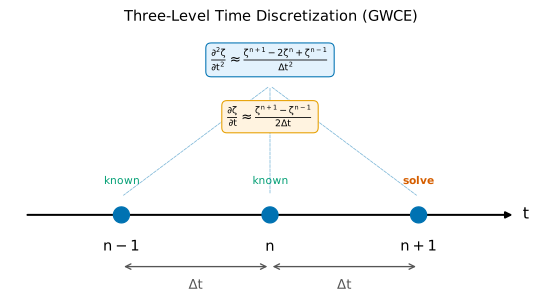
Fig. 36 Three-level time discretization stencil. The second-order temporal derivative uses values at all three levels; the first-order derivative uses the outer two.

\[\frac{\partial^2 \zeta}{\partial t^2} \approx \frac{\zeta^{n+1} - 2\zeta^n + \zeta^{n-1}}{\Delta t^2}\]

\[\frac{\partial \zeta}{\partial t} \approx \frac{\zeta^{n+1} - \zeta^{n-1}}{2\Delta t}\]

The RHS assembly in GwceVectorAssemblyKernels.hpp computes:

\[RHS_i = \text{(temporal)} + \text{(gradient)} + \text{(momentum)}\]

where:

• Temporal term: \(\frac{A_e}{12\Delta t}\left(\frac{1}{\Delta t} - \frac{\tau_0}{2}\right)(\zeta^n - \zeta^{n-1})\)

• Gradient terms: from \(c_{00}\) and \((a_{00}+b_{00})\) coefficients

• Momentum term: \(\nabla \cdot \mathbf{J}\)

Wet/Dry Integration

The GWCE assembly iterates over a pre-built wet-element list rather than checking wet/dry status inline. There is one such list per element type, reached as wet_indices<Elem>(), built by wetdry_build_wet_element_list<Elem>() after each wet/dry computation and containing only elements that are Active with all their vertices Wet (Wetting and Drying). The assembly is one function templated on the element-type tag, launched once per type into the same LHS/RHS; on a mesh without a type, that type’s list is never built and its launch never happens.

Dry nodes have their matrix row set to EP * delta_zeta = 0, preserving elevation unchanged.

Boundary Conditions

Dirichlet (Elevation-Specified):

For open boundary nodes with prescribed elevation \(\zeta_{bc}\):

1. Zero the matrix row except diagonal (set to EP)

2. Save off-diagonal coefficients for RHS modification

3. Set RHS to EP * (zeta_bc - zeta_current)

The elevation penalty (EP) is computed as the RMS of diagonal entries to maintain numerical conditioning.

Flow Boundaries:

Flow boundary conditions (types 22, 30, 32, 52) and weir boundary conditions (types 3, 13, 23, 4, 24) contribute to the GWCE RHS through a boundary integral term.

For each flow boundary node, a forcing quantity \(Q_{\text{force}}\) is computed. For type 22 (specified flux only):

\[Q_{\text{force},i} = \frac{q_n^{n+1} - q_n^{n-1}}{2\Delta t} + \tau_0 \, q_n^n\]

where \(q_n\) is the normal flux per unit width at the boundary node.

For types 30 and 32 (with Sommerfeld radiation):

\[Q_{\text{force},i} = \frac{q_n^{n+1} - q_n^{n-1}}{2\Delta t} - c \frac{2\,\Delta\zeta^{n} - (\zeta_E^{n+1} - \zeta_E^{n-1})}{2\Delta t} + \tau_0 \left( q_n^n - c \left( \zeta^n - \zeta_E^n \right) \right)\]

where:

• \(c = \sqrt{gH}\) is the shallow water wave celerity

• \(\Delta\zeta^n = \zeta^n - \zeta^{n-1}\) is the elevation increment from the previous GWCE solve

• \(\zeta_E\) is the prescribed elevation at the boundary

• \(H = h + \zeta\) is the total water depth

The \(2\Delta\zeta^n\) term provides a second-order extrapolation of the model elevation to time level \(n+1\). The radiation terms (proportional to \(c\)) allow outgoing long waves to pass through the boundary without reflection, following the Sommerfeld radiation condition.

\(Q_{\text{force}}\) is then applied to the GWCE RHS via boundary segment integration. For each segment connecting nodes \(i\) and \(j\):

\[\text{RHS}(i) \mathrel{+}= \frac{L_{2/3}}{4} \left( 2\,W_i Q_{\text{force},i} + W_j Q_{\text{force},j} \right)\]

\[\text{RHS}(j) \mathrel{+}= \frac{L_{2/3}}{4} \left( 2\,W_j Q_{\text{force},j} + W_i Q_{\text{force},i} \right)\]

where \(L_{2/3} = \tfrac{2}{3} L\) is the segment length scaled by 2/3. The 2:1 weighting arises from the linear basis function integration over the boundary segment. Wet/dry masking is applied: contributions are zeroed if either endpoint node is dry.

Map factors on the boundary integral. \(W\) is the endpoint’s map weight,

\[W = \sqrt{ \text{SFCX}^2 n_x^2 + \left( \text{SFCY} \cdot \text{YCFAC} \right)^2 n_y^2 }\]

evaluated with that node’s own scale factors and the outward normal \((n_x, n_y)\) of its boundary chord. The mapped GWCE multiplies the \(x\) and \(y\) flux divergences by \(\text{SFCX}\) and \(\text{SFCY}\cdot\text{YCFAC}\), so the boundary integral that closes the divergence theorem over the same mapped domain carries them too. Because \(\text{SFCX}\cdot\text{SFMY} = \text{SFCY}\cdot\text{YCFAC}\cdot\text{SFMX}\) for every projection Cocoa supports, the mapped boundary term is that common factor times the physical normal flux times physical arc length for any boundary orientation; \(W\) above is that statement rewritten on the projected normal and the projected arc length \(L\) actually measures, so it is exact at any latitude and any orientation. \(Q_{\text{force}}\) is a flux per physical metre, which is why the prescribed-discharge normalization below measures the boundary in physical metres as well.

Note

ADCIRC handles this differently, and it is worth stating precisely because Cocoa’s GWCE is otherwise term-for-term the same. In ADCIRC’s classic spherical mode (ICS = 2) the factors are simply absent from the boundary integral. In the cylindrical-mapping modes (ICS = 20 to 24) they are instead pre-multiplied into \(q_n\) itself, once at every read of the flux forcing (rotate_normal_flux in normal_flow_boundary.F90, called from cstart.F, hstart.F and timestep.F), as \(q_n \left( \text{SFCX}\cdot\text{SFMX}\, n_x^2 + \text{SFCY}\cdot\text{YCFAC}\, n_y^2 \right)\). That applies only to the prescribed-flux types 2, 12, 22 and 32 – never to weir or radiation boundaries, which produce \(q_n\) from the solution and so never pass through that routine – and the extra \(\text{SFMX}\) on the \(x\) term makes it inexact for an oblique boundary. Cocoa applies the weight in the integral instead, which covers every boundary type that produces \(Q_{\text{force}}\).

Weir Overflow (Types 3/13/23, 4/24):

Weir boundaries compute \(q_n\) dynamically from the overflow formula rather than prescribing it from a time series. Once \(q_n^{n+1}\) is determined, the standard QFORCE formula applies:

\[Q_{\text{force},i} = \frac{q_n^{n+1} - q_n^{n-1}}{2\Delta t} + \tau_0 \, q_n^n\]

External Weir (types 3/13/23):

External weirs have nodes on one side only. The overflow is always supercritical (free overflow), using only the source-side elevation:

\[h_f = \tfrac{2}{3}(\eta - z_{\text{crest}})\]

\[\begin{split}q_n = \begin{cases} -R \cdot C_p \cdot h_f \sqrt{h_f \cdot g} & \text{if } h_f > h_{\min} \\ 0 & \text{otherwise} \end{cases}\end{split}\]

where \(\eta\) is the water surface elevation at the boundary node, \(R\) is the ramp factor, and \(C_p\) is the supercritical discharge coefficient. The negative sign indicates outward flow (out of the domain).

Internal Weir (types 4/24):

Internal weirs have paired nodes on opposite sides of the crest. The overflow depends on the head difference between both sides and can be subcritical (submerged) or supercritical (free), flowing in either direction.

Given node A with elevation \(\eta_A\) and paired node B with elevation \(\eta_B\), define:

\[h_A = \eta_A - z_{\text{crest}}, \quad h_B = \eta_B - z_{\text{crest}}\]

\[h_{A,f} = \tfrac{2}{3} h_A, \quad h_{B,f} = \tfrac{2}{3} h_B\]

The overflow \(q_n\) is computed according to six regimes:

Case 1 — Both below crest (\(h_A \leq 0\) and \(h_B \leq 0\)):

\[q_n = 0\]

Case 2 — Equal levels (\(|h_A - h_B| < \delta_{\text{eq}}\)):

\[q_n = 0\]

Case 3 — Outward subcritical (\(h_A > h_B > h_{A,f}\) and \(h_A > h_{\min}\)):

\[q_n = -R \cdot h_B \cdot C_s \sqrt{2g(h_A - h_B)}\]

Case 4 — Outward supercritical (\(h_B \leq h_{A,f}\) and \(h_A > h_{\min}\)):

\[q_n = -R \cdot C_p \cdot h_{A,f} \sqrt{h_{A,f} \cdot g}\]

Case 5 — Inward subcritical (\(h_B > h_A > h_{B,f}\) and \(h_B > h_{\min}\)):

\[q_n = +R \cdot h_A \cdot C_s \sqrt{2g(h_B - h_A)}\]

Case 6 — Inward supercritical (\(h_A \leq h_{B,f}\) and \(h_B > h_{\min}\)):

\[q_n = +R \cdot C_p \cdot h_{B,f} \sqrt{h_{B,f} \cdot g}\]

where:

• \(R\) is the ramp factor

• \(C_s\) is the subcritical discharge coefficient

• \(C_p\) is the supercritical discharge coefficient

• \(h_{\min} = 0.04\) m is the minimum head threshold; no overflow occurs when the head above the crest is below this value

• \(\delta_{\text{eq}} = 0.01\) m is the equal-level tolerance; no overflow occurs when the head difference between sides is smaller than this

• Negative \(q_n\) indicates outward flow (A to B); positive indicates inward flow (B to A)

The transition between subcritical and supercritical occurs at a head ratio of 2/3, following standard weir hydraulics. Additionally, flow is blocked if the source side has no wet edges adjacent to the boundary node — for each weir node, the previous and next boundary nodes on the same side are checked for wet status, and if neither is wet the overflow is suppressed.

Lumped vs Consistent Mass Matrix

The solver type determines the solution strategy:

Fig. 37 GWCE solver flow for consistent and lumped variants

Cocoa supports two GWCE solver modes corresponding to ADCIRC’s ILUMP parameter:

Consistent Mass Matrix (ILUMP=0):

Uses the standard finite element mass matrix with off-diagonal coupling:

\[\text{OnDiag} = 2, \quad \text{OffDiag} = 1\]

This produces a sparse symmetric matrix that requires iterative solution (Conjugate Gradient with Jacobi preconditioning).

Lumped Mass Matrix (ILUMP=1):

Diagonalizes the mass matrix by summing each row to the diagonal:

\[\text{OnDiag} = 4, \quad \text{OffDiag} = 0\]

This produces a diagonal matrix allowing direct O(N) solution without iteration. The lumped approach trades some accuracy for significant computational savings.

Solver Type Selection:

The GwceSolverType enum controls which coefficients are used:

enum class GwceSolverType {
  Consistent,  // OnDiag=2, OffDiag=1 (ADCIRC ILUMP=0)
  Lumped       // OnDiag=4, OffDiag=0 (ADCIRC ILUMP=1)
};

Both the LHS (matrix, Equation (12)) and RHS (vector) assembly must use matching coefficients. The RHS temporal term uses:

\[\begin{split}\begin{split} RHS_i^{temp} = \bigl( &\text{OnDiag} \cdot \Delta\zeta_i \cdot S_i + \text{OffDiag} \cdot \textstyle\sum_{j \neq i} \Delta\zeta_j \cdot S_j \bigr) \\ &\cdot \frac{A_e}{12\Delta t} \left( \frac{1}{\Delta t} - \frac{\tau_0}{2} \right) \end{split}\end{split}\]

where \(S_i\) is the nodal scale factor (cos(latitude) for spherical coordinates).

Lumped Solver Performance:

The lumped solver eliminates iterative solve overhead but still requires:

1. RHS assembly (same complexity as consistent)

2. Diagonal solve: solution = RHS / diagonal using Tpetra built-ins

For optimal performance, boundary coefficient structures are cached at initialization rather than recreated each timestep.

On quadrilaterals. Both solver modes use the same OnDiag/OffDiag coefficient values, but a quadrilateral has no closed form to weight by them: the consistent path multiplies the integrated \(M_{ij}\) by \(S_j\) directly, and the lumped path adds the lumped row \(ML_i \cdot S_i\) with the same \(\tau_0/\Delta t\) factors as the triangle row sum – see the lumping convention.

Implementation Files

Consistent Solver:

• continuity/consistent/GwceSolverConsistent.hpp: Iterative CG solver

• continuity/consistent/GwceMatrixAssemblerConsistent.hpp: Full sparse matrix

• continuity/consistent/ConjugateGradientSolver.hpp: Belos CG wrapper

Lumped Solver:

• continuity/lumped/GwceSolverLumped.hpp: Direct diagonal solver

• continuity/lumped/GwceMatrixAssemblerLumped.hpp: Diagonal-only assembly

• continuity/lumped/GwceSolverLumpedKernels.hpp: Solve and update kernels

Shared:

• continuity/GwceVectorAssembler.hpp: RHS assembly (parameterized by solver type)

• continuity/GwceVectorAssemblyKernels.hpp: RHS assembly kernels

• continuity/OpenBoundaryCoefficients.hpp: BC coefficient storage

Quadrilateral only (reached only when the mesh has quadrilaterals):

• geometry/ReferenceElement.{hpp,cpp}, geometry/ElementGeometry.hpp, geometry/ElementTables.hpp: reference element, element geometry and device storage, shared by both element types (Quadrilateral Elements)

• continuity/ElementAssemblyMap.{hpp,cpp}: the CSR position of every entry of every 4x4 block, found once at assembler construction so the assembly kernel adds into the matrix without searching its rows

Every other file above is shared: the consistent LHS, the lumped LHS, the RHS assembly, the lateral-stress preprocessing and the slope limiter are one tag-templated body each, with a launch per element type.