Meteorological Forcing

Cocoa supports atmospheric forcing from wind fields and surface pressure data for storm surge and other weather-driven simulations. Forcing data is read from external files, interpolated onto the computational mesh, and applied at each timestep.

Overview

Meteorological forcing in Cocoa includes two components:

• Wind stress: Surface drag from 10-meter wind velocity, computed via the Garratt (1977) bulk drag law

• Atmospheric pressure gradient: Barotropic forcing from spatially varying surface pressure

Both components are read together from the same source and share a common temporal interpolation framework. A run may also combine several sources – of the same or different file formats – into one composed forcing field; see Composing Multiple Sources. See Meteorological Forcing for the mathematical formulation.

To generate the wind and pressure field analytically from a storm track instead of (or in addition to) gridded data, see Parametric Vortex (GAHM).

Any gridded source above can also carry sea-ice concentration, which attenuates wind stress in ice-covered water. It is opt-in and off by default: ice in a file is ignored unless forcing.meteorological.ice: true is set. See Ice Concentration.

Supported File Formats

Cocoa supports four meteorological file formats through the cocoa_meteo library:

Format	Config Value	Domains	Description
CF-compliant NetCDF	cf_netcdf	Single	Standard climate/forecast NetCDF with configurable variable names
OWI ASCII	owi_ascii	Multiple	ADCIRC-compatible paired pressure/wind ASCII files
OWI NetCDF	owi_netcdf	Multiple	NetCDF variant of OWI with support for moving (vortex-tracking) grids
GRIB2	grib	Multiple	Operational weather products (GFS, HRRR, RRFS, NAM, HWRF, HAFS) read directly via ecCodes; requires a build with -Dcocoa_ENABLE_GRIB=ON

The synonyms cf and netcdf (for cf_netcdf), owi (for owi_ascii), and grib2 (for grib) are also accepted.

Configuration

Meteorological forcing is configured in the forcing.meteorological section of the YAML configuration file.

Enabling Meteorological Forcing

To enable meteorological forcing, set enabled: true and specify the file format and path(s):

forcing:
  meteorological:
    enabled: true
    format: cf_netcdf
    filename: "path/to/meteo_data.nc"
  ramp:
    enabled: true
    duration: 1d

The ramp section controls the global spinup ramp applied to both tidal and meteorological forcing. To use a different ramp for meteorological forcing, add an optional ramp subsection under forcing.meteorological:

forcing:
  ramp:
    enabled: true
    duration: 5d                      # Applied to tidal forcing
  meteorological:
    enabled: true
    format: cf_netcdf
    filename: "path/to/meteo_data.nc"
    ramp:                           # Optional: overrides forcing.ramp for met
      enabled: true
      duration: 1d                     # Shorter met ramp

When the forcing.meteorological.ramp section is absent, the global ramp is used for both tidal and meteorological forcing.

CF NetCDF Format

forcing:
  meteorological:
    enabled: true
    format: cf_netcdf
    filename: "path/to/meteo_data.nc"

Optional variable name overrides:

By default, Cocoa expects the following NetCDF variable names. Override them under a nested variables map if your data uses different conventions:

Key	Default	Description
pressure	mslp	Mean sea level pressure variable name
wind_u	wind_u	Eastward 10-m wind component
wind_v	wind_v	Northward 10-m wind component
time	time	Time coordinate variable
lon	lon	Longitude coordinate variable
lat	lat	Latitude coordinate variable

Example with custom variable names:

forcing:
  meteorological:
    enabled: true
    format: cf_netcdf
    filename: "era5_data.nc"
    variables:
      pressure: "sp"
      wind_u: "u10"
      wind_v: "v10"
      time: "time"
      lon: "longitude"
      lat: "latitude"

OWI ASCII Format

OWI ASCII uses paired pressure and wind files per domain. This is the traditional ADCIRC meteorological forcing format.

Single domain:

forcing:
  meteorological:
    enabled: true
    format: owi_ascii
    filenames:
      - pressure: "path/to/fort.221"
        wind: "path/to/fort.222"

Multiple nested domains:

forcing:
  meteorological:
    enabled: true
    format: owi_ascii
    filenames:
      - pressure: "path/to/basin.pre"
        wind: "path/to/basin.wnd"
      - pressure: "path/to/region.pre"
        wind: "path/to/region.wnd"

Domain 0 (first entry) is the outer coarse grid. Subsequent entries are progressively finer inner grids. Where grids overlap, the innermost valid domain takes priority. Domains may also differ in time coverage; see Domain Time Windows.

OWI NetCDF Format

OWI NetCDF stores all domains in a single NetCDF file using group-based organization. It additionally supports moving (vortex-tracking) grids where the grid coordinates change at each time step.

forcing:
  meteorological:
    enabled: true
    format: owi_netcdf
    filename: "path/to/meteo_owi.nc"

GRIB2 Format

The GRIB reader ingests operational GRIB2 products directly – individual per-cycle snapshot files (each holding one valid time) or files carrying several times. At startup every file’s message headers are scanned and indexed by valid time, so filename order does not matter; incomplete or duplicated fields, grid changes within a domain, and misaligned time axes are all rejected with a descriptive error before the simulation starts.

GRIB support is compiled in with -Dcocoa_ENABLE_GRIB=ON, which requires an installed ECMWF ecCodes (point CMake at it with -Deccodes_DIR). ecCodes must be built with the JPEG2000 and CCSDS/AEC codecs that NCEP products use – spack install eccodes +memfs +aec jp2k=openjpeg provides a suitable build – and cocoa verifies those codec features are present at configure time (see Installation). GRIB2 fields are self-describing SI (Pa, m/s): pressure_scale is rejected for this format.

Single domain (GFS):

forcing:
  meteorological:
    enabled: true
    format: grib
    product: gfs
    filenames:
      - "gfs.t00z.pgrb2.0p25.f000"
      - "gfs.t00z.pgrb2.0p25.f003"
      - "gfs.t00z.pgrb2.0p25.f006"

The product preset selects which GRIB2 fields provide mean sea level pressure and 10-m winds. Available presets: gfs, hrrr, rrfs, nam, hwrf, hafs. GFS, NAM, HWRF, and HAFS use WMO-standard PRMSL; HRRR carries only the NCEP-local MSLMA reduction and RRFS only the NCEP-local MSLET (membrane) reduction, so those presets select the local parameters. NCEP files that pack the 10-m wind pair as a single multi-field GRIB message (e.g. NAM awphys) are handled transparently.

These products are 10-m winds from models that resolve land effects, so a mesh-based land wind reduction usually should not be applied on top: set wind_reduction: false at the meteorological level to leave the gridded field unreduced while, e.g., a composed parametric vortex is still reduced (see Per-source application).

Multiple GRIB resolutions (HRRR nested inside GFS), or GRIB mixed with another format:

Nesting a fine product inside a coarser one, or composing GRIB with a different format entirely, uses the general domains: list – each entry is a self-contained source with its own format (grib here, on every entry):

forcing:
  meteorological:
    enabled: true
    domains:
      - format: grib
        product: gfs          # domain 0: outer/coarse
        filenames: ["gfs_f000.grib2", "gfs_f001.grib2"]
      - format: grib
        product: hrrr         # domain 1: inner/fine, wins where it covers
        filenames: ["hrrr_f00.grib2", "hrrr_f01.grib2"]

See Composing Multiple Sources for the self-containment rule, coverage priority, and per-entry wind_reduction. Domains need not share a time step or phase – see Domain Time Windows.

A long forecast’s file list runs to hundreds of entries and is reusable across runs, so any filenames list (flat form or a domains entry) may instead be pulled from an external YAML file with an include node (see Configuration for the inclusion rules):

filenames:
  include: hafs_ida_files.yaml   # a YAML list of file paths

Regular latitude-longitude grids (GFS, HAFS parent domains) are handled natively, including global longitude wrapping and regional grids whose span crosses the antimeridian (routine for Pacific HAFS storms); projected grids (HRRR/RRFS/NAM Lambert conformal) are expanded to per-point coordinates and interpolated with the same inverse-bilinear machinery as irregular OWI grids. Bitmap-masked cells (missing data, e.g. outside a HAFS domain’s integration footprint) make the affected area fall through to the next-coarser domain.

Storm-following (moving) nests – the HWRF/HAFS storm output, where a fixed-shape regular grid translates with the storm each forecast hour – are detected automatically and handled by the same Lagrangian storm overlay used for OWI moving vortex grids (the grid origin is advected between snapshots and winds are blended magnitude-preserving, avoiding eye-wall vector cancellation). A moving nest may only change position: dimension, spacing, or projection changes are rejected, so a domain’s file list must come from a single forecast cycle. Moving nests must be regular lat-lon grids; a typical hurricane setup lists three domains, coarsest first (each entry still needs its own format: grib, like every domains: entry):

domains:
  - format: grib
    product: gfs
    filenames: [...]
  - format: grib
    product: hafs   # fixed parent domain
    filenames: [...]
  - format: grib
    product: hafs   # moving storm nest, highest priority
    filenames: [...]

For products the presets do not cover, the three fields can be selected explicitly by their numeric GRIB2 identity (shown here with the HRRR MSLMA values); level defaults to 0:

forcing:
  meteorological:
    enabled: true
    format: grib
    filenames: ["custom.grib2"]
    variables:
      pressure: {discipline: 0, category: 3, number: 198, surface_type: 101}
      wind_u:   {discipline: 0, category: 2, number: 2, surface_type: 103, level: 10}
      wind_v:   {discipline: 0, category: 2, number: 3, surface_type: 103, level: 10}

The same variables block may be given on a domains: entry (which still needs its own format: grib, like any other entry). surface_type is GRIB2 code table 4.5 (101 = mean sea level, 103 = height above ground).

Composing Multiple Sources

More than one meteorological source can drive a run at once – a basin-scale OWI background overlaid by a fine HAFS storm nest, or a GFS background with a GRIB HRRR inset – by listing them under forcing.meteorological.domains instead of the flat top-level keys used above. Each list entry is a fully self-contained source: it declares its own format and every key that format needs (files, product/variables for GRIB, wind_scale, pressure_scale, wind_reduction), so sources of different formats compose freely:

forcing:
  meteorological:
    enabled: true
    domains:
      - format: owi_ascii
        filenames:
          - pressure: "basin.pre"
            wind: "basin.wnd"
      - format: grib
        product: hafs
        filenames: ["hafs_storm_f00.grib2", "hafs_storm_f01.grib2"]

domains: cannot be combined with any top-level source key (format, filename/filenames, product, variables, wind_scale, pressure_scale, wind_reduction) – entries are self-contained, so there is nowhere else for that configuration to apply. In particular, format: grib at the top level combined with domains: is a startup error naming the offending key:

forcing.meteorological.domains cannot be combined with the top-level
'format' key; move the configuration into the domains entries

List order is coverage priority: entry 0 is the outermost/coarsest source, and later entries win at any node they cover (the same last-wins rule OWI’s own nested domains use, see OWI ASCII Format). A node not covered by any entry falls back to the ambient background (101300 Pa pressure, zero wind). The vortex block, if present, composes on top of whatever the domains: list produces exactly as it does over the flat form (Domains with a vortex below), unchanged – see Parametric Vortex (GAHM).

Per-entry wind_reduction

Each entry carries its own wind_reduction flag (default true, the same default as the flat form), so co-located sources can be corrected differently. A common pattern is a marine 10 m HAFS nest that still needs the land wind reduction, laid over an OWI background that is already a corrected surface wind and should not be reduced again:

forcing:
  meteorological:
    enabled: true
    domains:
      - format: owi_ascii        # basin-scale background, already a
        wind_reduction: false    # surface wind -- do not reduce again
        filenames:
          - pressure: "basin.pre"
            wind: "basin.wnd"
      - format: grib             # fine marine storm nest
        product: hafs
        wind_reduction: true     # reduce to a land wind where it covers
        filenames: ["hafs_storm_f00.grib2", "hafs_storm_f01.grib2"]

The flag is resolved per node from whichever entry actually covers it (the winner of the spatial combine), so a node under the HAFS nest is reduced even while a node left uncovered by it – and served by the OWI background – is not. See Per-source application for how the flag composes with the mesh’s roughness/canopy attributes, and Domain Time Windows for how sources with different time steps compose.

Domains with a vortex

A hurricane setup combining an OWI ASCII basin-scale background, a fine HAFS GRIB storm nest, and the GAHM parametric vortex – the full innermost-wins stack, gridded reader composition plus the vortex layered on top:

forcing:
  meteorological:
    enabled: true
    domains:
      - format: owi_ascii          # basin-scale background: already a
        wind_reduction: false      # surface wind, so leave it unreduced
        filenames:
          - pressure: "basin.pre"
            wind: "basin.wnd"
      - format: grib               # fine marine 10 m storm nest: reduce
        product: hafs               # it to a land wind where it covers
        wind_reduction: true
        filenames: ["hafs_storm_f00.grib2", "hafs_storm_f01.grib2"]
    vortex:
      model: gahm
      tracks:
        - "storm_bal.dat"
      wind_reduction: true          # the vortex is also a marine wind
  ramp:
    enabled: true
    duration: 1d

The HAFS nest and the OWI background can each be produced on their own native cadence (Domain Time Windows) – neither has to be resampled to match the other or the vortex’s per-snapshot track times. Both gridded sources reduce or not per their own physical nature (the OWI background is already surface-level; the HAFS nest and the vortex are both marine winds that need the mesh’s land correction), independent of composition order.

Activation Ramp

A domains: entry’s data window, or a vortex track’s own start/end, does not have to span the whole simulation – a fine HAFS storm nest may only start at hour 48, arriving against an ocean that has already spun up but is still storm-free. By default that arrival is a hard edge: the source comes in over a single data interval (Domain Time Windows), which for an intense, coarsely-sampled nest can still look like a step to the rest of the composed field.

Each domains: list entry – not the flat top-level source, which has no window of its own – and the vortex: block accept a ramp: <duration> key (e.g. 6h; default 0, off) that smooths this into an explicit cross-fade. The fade is a composition blend, not a scale on the source’s own values: at every node it interpolates between the composed field without that source and the composed field with it,

node = (1 - w) * underlying + w * source

with the weight w ramping from 0 to 1 as the window opens and back to 0 as it closes, symmetrically, using the same normalized tanh(2t/T) / tanh(2) shape as the top-level cold-start ramp block (Combining Meteorological and Tidal Forcing) – one curve shared by both uses so they cannot drift apart. Because the two sides of the blend already agree everywhere outside the source’s own spatial coverage, the fade is spatially seamless: it cannot introduce a seam at a nest boundary, and the composed field can never dip below the underlying data, unlike a plain scale on the source.

The fade is symmetric: the same duration applies at window-open and at window-close, each referenced to that edge’s own time. A window shorter than twice the ramp duration never reaches full weight – the fade-in and the fade-out are both still in progress when the other edge arrives – which is deliberate, not an error: a very short-lived nest fades smoothly in and back out rather than plateauing at full weight.

forcing:
  meteorological:
    enabled: true
    domains:
      - format: owi_ascii
        filenames:
          - pressure: "basin.pre"
            wind: "basin.wnd"
      - format: grib
        product: hafs
        ramp: 6h                 # cross-fade in/out over the nest's own window edges
        filenames: ["hafs_storm_f00.grib2", "hafs_storm_f01.grib2"]

See Vortex Configuration for the equivalent vortex.ramp key, which fades a storm in and out against its own track’s first and last snapshot times rather than a data window.

The full stack: a worked storm configuration

Everything above composes in a single run. This configuration layers four gridded sources of three formats, two parametric storms, and every kind of ramp the model has – each doing a different job on a different clock:

forcing:
  meteorological:
    enabled: true

    # Model cold-start spinup: ONE ramp for the whole composed field,
    # referenced to the start of the meteorological data. Protects the
    # quiescent ocean at initialization; unrelated to the per-entry
    # activation ramps below.
    ramp:
      enabled: true
      duration: 12h

    domains:
      # Layer 0: basin-scale OWI background spanning the whole run.
      # Already a corrected surface wind, so opt out of the land
      # reduction. Present from t=0, so it needs no activation ramp.
      - format: owi_ascii
        wind_reduction: false
        filenames:
          - pressure: "basin.pre"
            wind: "basin.wnd"

      # Layer 1: regional GFS on its own (coarser) cadence. Marine
      # 10 m wind: leave wind_reduction at its default (true). Its
      # files start a day into the run, so fade it in over 3 hours
      # instead of stepping in at its first snapshot.
      - format: grib
        product: gfs
        ramp: 3h
        filenames: ["gfs_f000.grib2", "gfs_f003.grib2", "gfs_f006.grib2"]

      # Layer 2: fixed HAFS parent domain around the storm basin.
      - format: grib
        product: hafs
        ramp: 6h
        filenames: ["hafs_parent_f00.grib2", "hafs_parent_f01.grib2"]

      # Layer 3: the moving HAFS storm nest, produced only around
      # landfall. The reader detects the translating grid from the
      # files; the 6 h ramp cross-fades its arrival and departure.
      - format: grib
        product: hafs
        ramp: 6h
        filenames: ["hafs_nest_f00.grib2", "hafs_nest_f01.grib2"]

    # Innermost: the parametric vortex, layered over whatever the
    # domains produce. Two storms, applied in list order (the later
    # track wins where they overlap). The single vortex ramp fades
    # EACH storm against its own track's first/last snapshot times,
    # so the two storms fade in and out independently.
    vortex:
      model: gahm
      tracks:
        - "storm_a.dat"
        - "storm_b.dat"
      ramp: 6h
      wind_reduction: true

Three kinds of ramp appear in that file, and they never share a clock:

Key	Clock	What it fades
meteorological.ramp	The model cold start (one reference time for the run)	The entire composed field – wind, stress, and the pressure anomaly about the ambient background – during spinup (Combining Meteorological and Tidal Forcing)
domains[i].ramp	Each of that entry’s data windows on the union time axis	That source’s arrival and departure, cross-faded against the field composed without it (Activation Ramp)
vortex.ramp	Each storm track’s own first and last snapshot times	Each storm’s overlay weight, independently per track (Vortex Configuration)

Every gridded source above may also run on its own cadence – 15-minute OWI, 3-hourly GFS, hourly HAFS – with no resampling (Domain Time Windows), and the per-node land reduction follows whichever entry wins each node (Per-entry wind_reduction).

Domain Time Windows

Domains need not cover the same period or share a time step: each domain (an OWI ASCII file pair, an OWI NetCDF group, or a domains: list entry) carries its own time axis covering only the window it has data for. A typical layout pairs a basin-scale grid spanning the whole simulation with a fine storm grid produced only around landfall.

Cocoa builds the sorted union of every domain’s own times. At a union time that is exactly one of a domain’s own samples, that domain’s data is used verbatim (an exact-match short-circuit); at a union time strictly between two of a domain’s own samples, its pressure and wind are linearly interpolated from that domain’s own bracketing snapshots. A domain’s sample rate therefore never has to match another’s – an hourly HRRR nest composes with a 3-hourly GFS background with no configuration needed. A moving (storm-following) domain’s grid position is interpolated the same way, so a fine nest’s origin moves continuously between its own reported positions even while a coarser domain refills on a different cadence.

Outside its own window a domain is inactive: it contributes nothing, and its coverage falls through to the next outer domain or to the ambient background (background pressure, zero wind). By default the window edge is hard: the piecewise-linear interpolation between snapshots brings the domain in over a single data interval, which for a coarse cadence (a 3- or 6-hourly nest) can still look like a step to the rest of the composed field. Each domains: entry (and the vortex: block) can smooth this into an explicit, configurable-duration cross-fade with its own ramp key – see Activation Ramp – off by default, so the hard edge described above is unchanged unless configured.

Each domain’s data window is reported in the log at startup (debug level), and during the run each domain announces when the simulation first enters and leaves its window. A domain whose window never overlaps the simulated period produces a warning. The same announcements are made for each parametric vortex track (see Composed with a gridded background).

Drag Law

The wind drag law used to convert 10-m wind velocity to surface stress is selected with forcing.meteorological.drag_law. The only accepted value is garratt (the Garratt 1977 bulk drag law), which is also the default:

forcing:
  meteorological:
    enabled: true
    format: cf_netcdf
    filename: "data.nc"
    drag_law: garratt   # default; only accepted value

Scale Factors

Cocoa applies configurable scale factors to convert raw file values to SI units (Pa for pressure, m/s for wind):

Parameter	Default	Description
pressure_scale	100.0	Multiplier for pressure values. Default converts hectopascals (hPa) to pascals (Pa).
wind_scale	1.0	Multiplier for wind velocity values. Default assumes m/s input.

Example for a dataset with pressure in Pa and wind in knots:

forcing:
  meteorological:
    enabled: true
    format: cf_netcdf
    filename: "data.nc"
    pressure_scale: 1.0        # Already in Pa
    wind_scale: 0.514444       # Convert knots to m/s

File Format Details

CF-Compliant NetCDF

The CF NetCDF reader expects a regular rectangular grid with the following structure:

Required dimensions and variables:

dimensions:
  time = UNLIMITED ;
  lat = <NY> ;
  lon = <NX> ;

variables:
  double time(time) ;
    time:units = "hours since 2026-01-01 00:00:00" ;
    time:calendar = "standard" ;
  double lat(lat) ;
  double lon(lon) ;
  float mslp(time, lat, lon) ;    // Surface pressure
  float wind_u(time, lat, lon) ;  // Eastward 10-m wind
  float wind_v(time, lat, lon) ;  // Northward 10-m wind

• The time variable must use CF-compliant units (e.g., "hours since ..." or "seconds since ...")

• Longitude and latitude are 1D coordinate arrays defining the grid

• Global grids (360° longitude span) are detected automatically; the reader handles wrap-around

OWI ASCII

OWI ASCII files use a fixed-width format with one pressure file and one wind file per domain.

File header (line 1):

Oceanweather WIN/PRE Format                            YYYYMMDDHH  YYYYMMDDHH

The header line contains a format identifier, the start time, and the end time.

Snapshot header (one per time step):

iLat= NNNiLong= NNNdx=D.DDDDdy=D.DDDDSWLat=LL.LLLLLSWLon=LLL.LLLLDT=YYYYMMDDHHNN

Field	Position	Description
iLat	cols 5-8	Number of latitude points (NY)
iLong	cols 15-18	Number of longitude points (NX)
dx	cols 22-27	Longitude grid spacing [degrees]
dy	cols 31-36	Latitude grid spacing [degrees]
SWLat	cols 43-50	Southwest corner latitude [degrees]
SWLon	cols 57-64	Southwest corner longitude [degrees]
DT	cols 68-79	Snapshot time (YYYYMMDDHHNN)

Data records:

Following each snapshot header, NX * NY floating-point values are written in free format. Pressure files contain one field per snapshot; wind files contain two fields (eastward U, then northward V).

OWI NetCDF

OWI NetCDF files use NetCDF groups to organize multi-domain data:

root group:
  dimensions:
    time = UNLIMITED ;
  variables:
    double time(time) ;

group: domain_0 {
  dimensions:
    node = <NX*NY> ;
  variables:
    double longitude(time, node) ;
    double latitude(time, node) ;
    float pressure(time, node) ;
    float wind_u(time, node) ;
    float wind_v(time, node) ;
}

group: domain_1 {
  ...
}

The per-domain coordinate arrays (longitude, latitude) vary with time, enabling vortex-tracking grids that follow a storm center. For stationary grids, the coordinates are the same at each time step.

Parametric Vortex (GAHM)

Cocoa can generate a tropical-cyclone wind and pressure field analytically from a storm track, instead of (or in addition to) reading gridded meteorological data. The parametric model is the Generalized Asymmetric Holland Model (GAHM) [Gao2013], an asymmetric extension of the classic Holland [Holland1980] profile that fits a separate radius-to-maximum-wind and Holland \(B\) shape parameter to each storm quadrant and each reported wind-speed isotach. The vortex is evaluated on the device (GPU or CPU) directly at the mesh nodes every time step, so no external wind file is required for a synthetic or best-track storm.

The vortex is the innermost meteorological “domain”. Inside the storm footprint it overlays whatever lies beneath it: a gridded background, the ambient constants, or a previously applied storm. At the edge it fades to the underlying field through a blend ring (see Blend ring). The resulting 10 m wind and sea-level pressure feed the same wind-stress and pressure-gradient forcing as gridded meteorology, including the ramp and the wind-reduction pipeline documented under Wind Reduction.

Theory

GAHM builds a per-quadrant wind and pressure field from a handful of track scalars by fitting a modified Holland profile that retains the Coriolis term. This section sketches the equations Cocoa evaluates; they live in cocoa_vortex/physics/GahmPhysics.hpp. Full derivations are in [Gao2013]; the underlying analytic wind and pressure profile is the Holland model [Holland1980] and its revision [Holland2010].

Holland profile and its limitation

The classic Holland [Holland1980] model sets the profile shape from a single parameter

\[B = \frac{\rho_a\, e\, v_\mathrm{max}^2}{\Delta p}, \qquad \Delta p = p_n - p_c,\]

with air density \(\rho_a\), Euler’s number \(e\), and the pressure deficit \(\Delta p\) between the environmental pressure \(p_n\) and the central pressure \(p_c\). Its wind follows from cyclostrophic balance, which sets the pressure gradient against the centrifugal force alone. Dropping the Coriolis term is accurate near the eyewall of an intense storm but degrades the fit far from the center and for weak or large storms, where rotation is not negligible.

Gradient-wind generalization

GAHM restores gradient-wind balance (pressure gradient against centrifugal and Coriolis force). The relative importance of rotation is the Rossby number

\[\mathrm{Ro} = \frac{v_\mathrm{max}}{|f|\, R_\mathrm{max}},\]

where \(f = 2\Omega\sin(\mathrm{lat})\) is the Coriolis parameter (the scalar physics uses its magnitude \(|f|\)). A scaling parameter \(\varphi\) and a modified shape parameter \(B_g\) then generalize Holland’s \(B\):

\[\varphi = 1 + \frac{1}{\mathrm{Ro}\,B_g\,(1 + 1/\mathrm{Ro})}, \qquad B_g = B\,\frac{(1 + 1/\mathrm{Ro})\,e^{\varphi - 1}}{\varphi}.\]

The two are coupled (\(\varphi\) depends on \(B_g\) and vice versa), which is why the fit iterates (below). As \(|f| \to 0\) (the equator, or the cyclostrophic limit) \(\mathrm{Ro} \to \infty\), \(\varphi \to 1\), and \(B_g \to B\), so GAHM reduces to Holland exactly. Cocoa returns these limits explicitly near the equator rather than dividing by \(|f|\).

The gradient wind actually evaluated, at radius \(r\) with \(a = R_\mathrm{max}/r\), is

\[V_g(r) = \sqrt{\,v_\mathrm{max}^2\,\bigl(1 + \tfrac{1}{\mathrm{Ro}}\bigr)\, e^{\,\varphi\,(1 - a^{B_g})}\,a^{B_g} + \Bigl(\tfrac{r|f|}{2}\Bigr)^{2}} \;-\; \frac{r|f|}{2},\]

and the surface pressure is

\[p(r) = p_c + (p_n - p_c)\,e^{-\varphi\,(R_\mathrm{max}/r)^{B_g}}.\]

\(V_g\) is the boundary-layer wind; the 10 m wind and the final wind vector (frictional inflow turning, translation, and a fixed frame rotation) are assembled from it (see Ten-minute wind and Translation asymmetry).

Per-quadrant isotach fit

A track snapshot reports, per quadrant, the radius at which the wind falls to each standard isotach (34/50/64 kt). GAHM treats every (quadrant, isotach) pair independently: \((R_\mathrm{max}, B_g, \varphi)\) are chosen so the gradient wind passes through the reported isotach speed \(v_i\) at the reported isotach radius \(r_i\),

\[V_g(r_i;\, R_\mathrm{max}, B_g, \varphi) = v_i.\]

Cocoa solves this once per snapshot at startup: an inner bracketed Newton iteration on \(R_\mathrm{max}\) over \((0, r_i]\) (the wind is monotone in \(R_\mathrm{max}\) there, so a step leaving the bracket is halved toward the bound), wrapped in an outer fixed-point iteration that updates \(B_g\) and recomputes \(\varphi\) from it until \(B_g\) stops changing. Because the profile is constructed to pass through each isotach, the wind it produces recovers the reported isotach speed at the reported radius by construction. This is the isotach-recovery property the Verification workflow checks.

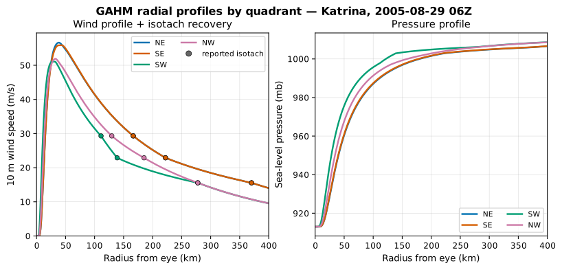
Fig. 4 GAHM radial profiles for Hurricane Katrina at its 2005-08-29 06Z near-landfall snapshot, evaluated by Cocoa’s own device-callable physics on a set of radial points. Left: the 10 m wind rises to a peak at \(R_\mathrm{max}\) (~30 km) and decays outward. The markers are the reported NHC 34/50/64 kt isotachs; the isotach-recovery property holds by construction, so every curve passes exactly through its isotach at \(0.89\times\) the reported one-minute speed (the ten-minute equivalent). The four quadrants differ (NE/SE reach 34 kt near 370 km, SW near 278 km): the storm is asymmetric. Right: the pressure rises monotonically from the central pressure (~913 mb) toward the environmental pressure, faster in the more compact SW/NW quadrants.

Azimuthal composition

The four quadrant solutions are stitched into a field continuous in azimuth. At a bearing whose blend angle from one quadrant toward the next is \(\theta \in [0, \tfrac{\pi}{2}]\), each solved parameter \(X\) is an inverse-square-weighted average of its two bounding-quadrant values:

\[X(\theta) = \frac{w_1 X_1 + w_2 X_2}{w_1 + w_2}, \qquad w_1 = \frac{1}{\theta^2},\quad w_2 = \frac{1}{(\pi/2 - \theta)^2}.\]

The weighting pulls the field to the pure quadrant value on each quadrant centerline (\(\theta = 0\) or \(\pi/2\)); Cocoa returns the exact bounding value within a small tolerance of a centerline to avoid the division-by-zero the raw weights have there. The same weighting sets the azimuthal coverage radius \(R_\mathrm{out}(\theta)\) used by the Blend ring.

Translation asymmetry

A moving storm is asymmetric: its forward motion adds to the wind on one side and subtracts on the other. GAHM removes the storm-translation velocity \(\mathbf{U}_t\) from the reported winds before the fit and adds it back after evaluation, so the fit sees a quasi-stationary vortex. The removal is common to both methods below; they differ only in how much motion is removed and how it is re-added.

Removal is a vector quotient: the solver receives the reported quadrant isotach speed divided by the magnitude of the quadrant unit vector plus the normalized translation,

\[v_\mathrm{quad} = \frac{v_i} {\bigl\lVert \hat{\mathbf{u}} + \mathbf{U}_t / v_\mathrm{max} \bigr\rVert}.\]

Two re-addition conventions are selectable through env_wind; both follow the GAHM2026 reference [Gao2013] [Luettich2026].

ADCIRC (env_wind: adcirc, the default and Luettich’s recommendation) scales the translation by an empirical function of the eye-to-eye motion between consecutive snapshots,

\[\lVert \mathbf{U}_t \rVert = 1.5\, \left| \frac{\Delta s}{\Delta t} \right|^{0.63} \,(0.51444)^{0.37},\]

where the trailing \((0.51444)^{0.37}\) reconciles GAHM’s knots-based coefficient with the m/s eye motion (\(0.51444\) is the knot-to-m/s factor; without it the coefficient silently carries the wrong units). The translation is re-added scaled by the local-to-maximum wind ratio,

\[\mathbf{V}_\mathrm{env} = \mathbf{V} + \mathbf{U}_t\,\frac{\lVert \mathbf{V} \rVert}{v_\mathrm{max}},\]

so the asymmetry is strongest near the radius of maximum winds and fades in the weak outer field.

Lin & Chavez (env_wind: lin_chavez, [LinChavez2012]) removes a smaller fraction of the motion and re-adds it as a constant background vector rather than a profile-scaled one:

\[\lVert \mathbf{U}_t \rVert = 0.6\,\left| \frac{\Delta s}{\Delta t} \right|, \qquad \mathbf{V}_\mathrm{env} = \mathbf{V} + \mathcal{R}_{20^\circ}\,\mathbf{U}_t,\]

where \(\mathcal{R}_{20^\circ}\) rotates the translation vector \(20^\circ\) from the storm heading (toward the low, i.e. counterclockwise in the Northern Hemisphere and clockwise in the Southern, via \(\operatorname{sign}(\text{lat})\)). The constant re-add is applied only inside the storm footprint, so the ambient field outside the blend ring is untouched.

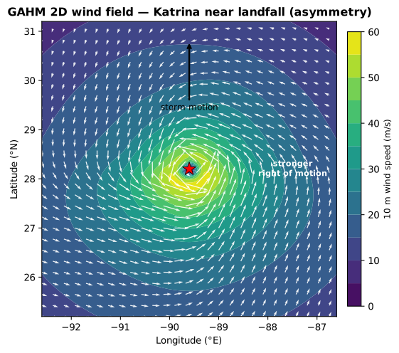
Fig. 5 The GAHM 2D wind field for the same Katrina snapshot, produced by solving the vortex on a structured longitude/latitude grid and plotting the result. The wind circulates counterclockwise about the eye (a Northern-Hemisphere storm); the arrows are the wind vectors and the fill is wind speed. The field is asymmetric: with the storm moving north, the translation adds to the wind on the right of motion (the eastern flank); together with the wider reported isotachs there, this makes the eastern half stronger and broader than the western half. A Southern-Hemisphere storm mirrors this, circulating clockwise (see Southern Hemisphere).

From theory to code

The fit runs on the host, once at startup, in cocoa_vortex/solver (GahmSolver and GahmPreprocessor): the Newton/fixed-point solve of \((R_\mathrm{max}, B_g, \varphi)\) per quadrant and isotach, plus the translation preparation. The closed-form evaluation lives in cocoa_vortex/physics/GahmPhysics.hpp as KOKKOS_INLINE_FUNCTION routines: gradient wind, pressure, azimuthal blend, and wind-vector assembly. The host reference evaluator and the device overlay kernel therefore call the same functions and agree to floating-point tolerance (see Solve-once, interpolate-packs).

Vortex Configuration

The vortex is configured under forcing.meteorological.vortex. Meteorological forcing may run with only a vortex, only a gridded reader, or both; enabled: true requires at least one of format/filename or vortex.

Key	Default	Description
model	gahm	Parametric model. gahm is the only accepted value.
tracks	(required)	Non-empty list of ATCF track files, applied in list order. Each is a best-track file or a preprocessed single-cycle forecast (see Forecast tracks).
blend_factor	1.25	Outer edge of the blend ring as a multiple of the outermost isotach radius. Must be \(\ge 1.0\).
wind_reduction	true	Apply the land wind-reduction corrections (directional roughness and canopy) to the vortex wind before it is blended. Defaults on: a parametric vortex is a marine 10 m wind that should be reduced to a land surface wind. Set false to leave it unreduced (e.g. when composing over a gridded field that already carries the reduction). Only takes effect when the mesh carries the reduction attributes. See Wind Reduction.
pressure_estimate	courtney_knaff_2009	Wind-pressure relationship used to fill a missing central pressure (forecast a-decks omit MSLP). One of courtney_knaff_2009, knaff_zehr_2007, dvorak_1984, atkinson_holliday_1977, or none (fail loud on a missing pressure). See Estimating a missing central pressure.
pressure_anchor_hours	48	Bias-offset anchoring window [h] that smooths the hindcast-to-forecast pressure seam in a combined best-track + forecast file. 0 disables anchoring (pure per-snapshot estimate).
env_wind	adcirc	Storm-motion (environmental wind) re-addition convention: adcirc (profile-scaled, the empirical GAHM re-add) or lin_chavez (constant background vector rotated \(20^\circ\)). See Translation asymmetry.
boundary_layer_factor	0.9	Gradient-wind-to-10 m boundary-layer reduction applied to the top-of- boundary-layer wind. Must lie in \([0.75, 0.9]\); 0.9 is the GAHM default. See Ten-minute wind.
ramp	0 (off)	Duration of the activation/deactivation cross-fade applied as each storm’s own track data window opens or closes (e.g. 6h), referenced to that track’s first and last snapshot times. Folded into the storm’s spatial blend ring (Blend ring) rather than a separate step. Distinct from the top-level forcing.ramp cold-start spinup ramp (see Combining Meteorological and Tidal Forcing), which fades the whole composed field in once at the start of the run; the equivalent per-source key for a gridded domains: entry is documented at Activation Ramp.

Vortex-only

With no format/filename, the provider runs in vortex-only mode: the vortex is overlaid on the ambient background pressure and zero wind.

forcing:
  meteorological:
    enabled: true
    vortex:
      model: gahm
      tracks:
        - "katrina_bal122005.dat"
      blend_factor: 1.25
  ramp:
    enabled: true
    duration: 1h

Composed with a gridded background

A gridded reader and a vortex can be combined. Where both are active the vortex rides on the interpolated gridded field; outside the gridded data’s time window the vortex still applies over the ambient background. The provider’s effective data window is the union of the reader window and the vortex track window.

Each gridded domain and each vortex track announces itself in the log when the simulation first enters and leaves its data window, so a run’s log records when each source was actually forcing the solution. A track whose window never overlaps the simulated period produces a warning.

forcing:
  meteorological:
    enabled: true
    format: cf_netcdf
    filename: "background_met.nc"
    vortex:
      model: gahm
      tracks:
        - "storm.dat"
      ramp: 6h                              # fade the storm in/out at its own track window edges
  ramp:
    enabled: true
    duration: 12h

Multiple storms

Listing more than one track overlays several storms in a single run. Storms are applied in list order, so a later entry wins in an overlap: inside a later storm’s footprint the earlier storm becomes the underlying field that the later storm blends against.

forcing:
  meteorological:
    enabled: true
    vortex:
      model: gahm
      tracks:
        - "storm_a.dat"   # underlying where they overlap
        - "storm_b.dat"   # wins the overlap

The optional ramp key applies per storm: each track fades in and out against its own first and last snapshot times, so two storms whose tracks cover different periods activate and retire independently even though they share the one configured duration.

Blend ring

Each storm has full weight inside R_out (the outermost, i.e. weakest, reported isotach radius, blended around the azimuth), then ramps linearly to zero weight at blend_factor * R_out and applies nothing beyond. This avoids a hard discontinuity at the storm edge. The blend against the underlying field is a plain linear interpolation of the wind components and pressure, which is correct when the underlying field may point in a different direction from the vortex wind.

When ramp (Vortex Configuration) is set, this same per-node ring weight is additionally multiplied by the storm’s own activation/deactivation cross-fade, referenced to the track’s first and last snapshot times. The entire footprint, out to the ring’s outer edge, fades in and out smoothly as the track’s window opens and closes.

Physics conventions

Ten-minute wind

ATCF best tracks report a one-minute maximum sustained wind. GAHM works in ten-minute winds, so the one-to-ten-minute conversion factor (0.89) is applied early, during track preprocessing, before the Rmax/\(B_g\) solve. Reported isotach wind speeds are treated consistently. The peak 10 m wind produced at the radius of maximum winds therefore tracks vmax * 0.89 * (boundary-layer factor) rather than the raw one-minute vmax.

The boundary-layer factor reduces the gradient (top-of-boundary-layer) wind to the 10 m wind. It is configurable through boundary_layer_factor over the physically defensible range \([0.75, 0.9]\); the default 0.9 is the GAHM value. Lower values within the range yield a weaker surface wind for the same gradient wind, and the reported-isotach recovery holds at any setting because the same factor is applied on both the removal and evaluation sides of the fit.

Southern Hemisphere

Southern-Hemisphere storms (negative latitude, SH basin) are supported: the Coriolis sign flips and the tangential wind sense reverses (clockwise rotation). The wind magnitude differs legitimately from the Northern- Hemisphere mirror because the translation-asymmetry preparation is itself hemisphere-dependent. Under env_wind: lin_chavez, the \(20^\circ\) storm-motion rotation follows \(\operatorname{sign}(\text{lat})\) and turns the opposite way in the two hemispheres.

Solve-once, interpolate-packs

For each track snapshot Cocoa solves the per-quadrant, per-isotach GAHM parameters once at preprocessing. Between snapshots it linearly interpolates the solved parameters (radius-to-max-wind, \(B_g\), the scaling parameter \(\varphi\)) and the storm scalars (eye position, central pressure, translation), rather than re-solving at every model time step. This is a deliberate, documented deviation from re-solving on every query: at a snapshot time the interpolation weight is 0 or 1, so evaluation reduces exactly to a single snapshot. The committed regression references are generated against exactly that single-snapshot state, so the deviation does not affect them. In MPI runs every rank preprocesses the (tiny) track identically, with no communication.

Track input (ATCF)

Tracks are comma-delimited ATCF files, one record per line. Cocoa parses the cycle time, forecast hour, eye position, one-minute vmax, central pressure, the pressure of the outermost closed isobar (RADP), the radius to maximum winds, and the wind-radii (34/50/64 kt) quadrant records. Best-track (b-deck) and forecast (a-deck) files share the same column layout; the differences that matter for Cocoa are called out under Forecast tracks. Key expectations:

• The forecast-hour column (tau, field 6) is added to the cycle time in whole hours, and the minutes column (field 4) is added within the hour, so both off-synoptic best-track times and multi-hour forecast lead times land on the correct valid time.

• Snapshot times must be strictly increasing; out-of-order lines are rejected (they would silently reverse the translation vector).

• Same-time lines are merged (multiple isotach records for one valid time); disagreeing storm scalars at the same time are a hard error.

• Short (fewer-than-28-column) lines are skipped with a warning, so wave-radii or other non-standard trailing records do not abort the run.

• The environmental pressure \(p_n\) comes from the RADP column (field 18), falling back to the 1013 mb standard atmosphere only when that column is blank or zero, as on older b-decks. This matters most for weak systems: a storm reported at 1012 mb with RADP = 1017 mb has a 5 mb deficit, not the 1 mb the standard atmosphere would imply.

• A quadrant radius of zero means the isotach was not reported there, not that it has zero size. Cocoa does not invent one; that quadrant’s radius-to-max-wind is filled after the solve from a neighbor (see Weak and incomplete tracks).

• B-decks routinely carry filler and genesis lines, so a snapshot missing its central pressure, vmax, or eye position is skipped with a warning rather than aborting the run. A track left with no usable snapshot at all fails loud.

• Cocoa rejects an already-preprocessed fort.22, i.e. the output of ADCIRC’s aswip (NWS 19/20) or of GAHM2026. Its first 28 columns are b-deck-compatible so it would otherwise parse cleanly, but its isotachs already have the environmental wind removed and it carries solved quadrant-Rmax and Holland-\(B\) columns; re-solving it would apply the whole preprocessing chain a second time. Supply the b-deck it was generated from.

Best-track files

The intended, drop-in input is a best-track (b-deck) file: one storm, technique BEST, tau = 0 on every line, chronological. NHC b-decks (e.g. bal122005.dat for Katrina) are used directly, no preprocessing required.

Weak and incomplete tracks

Real tracks are frequently incomplete: genesis and invest lines report no isotach at all, quadrant radii go missing, and a barely-closed system can be reported with a central pressure at or above its own environmental pressure. Cocoa follows GAHM2026’s consistency checks, which are designed to keep such a track usable rather than to reject it.

The shape parameter is clamped. Holland’s \(B\) scales as \(v_{\max}^2 / \Delta p\), so a weak system reported with a small deficit drives it far outside its physical range. \(B\) is clamped into \([0.5, 2.5]\) and the clamp is logged with the storm, time, wind, and deficit that produced it. This is what makes an unguarded deficit safe: a zero deficit sends \(B\) to infinity and a negative one sends it negative, and both land on a bound instead of in the solver.

A non-positive deficit is not rejected. If \(p_c \ge p_n\) the deficit is negative, \(B\) clamps to its lower bound, and the storm is evaluated with a shallow inverted pressure anomaly. This is deliberate parity with GAHM2026, which keeps such lines. Read the clamp warnings: a track that produces them throughout is telling you its pressures are not usable, even though the run completes.

Storms too weak to fit are not fit. Below a 20 kt maximum vortex speed at the top of the boundary layer, an isotach fit carries no information, and the radius-to-max-wind for the whole snapshot comes from the track’s reported RMW instead. The same applies per quadrant below a 5 kt vortex isotach speed.

Unreported radii are filled, never fabricated. A quadrant-isotach with no reported radius, one too weak to fit, or one whose fit failed takes its radius-to-max-wind from a neighbor: the 34 kt slot copies the next higher isotach of its own quadrant, and otherwise \(B\) is re-solved at the quadrant’s representative radius (the highest isotach that solved there, or the azimuthal mean when that quadrant solved nothing). Filled packs are marked in the parameter table’s solve status, so they are always distinguishable from fitted ones.

There is always a radius. When a snapshot solves nothing anywhere, the radius comes from the track’s reported RMW; when the track reports none either, from the last snapshot that produced one; and failing that from a 25 nmi default, matching aswip. A DUMY filler line at the head of a genesis track therefore costs nothing.

Forecast tracks

NHC also distributes forecast guidance as ATCF a-deck aid files (e.g. aal092021.dat). These share the b-deck column layout, and the tau column already does the right thing: a single forecast cycle expands to a sequence of snapshots at cycle time + 0, +12, +24 … hours, strictly increasing. A forecast a-deck is not a drop-in file. Prepare it in three steps.

1. Reduce to one technique and one cycle. An a-deck interleaves every objective aid (CARQ, AVNO, OFCL …) across every advisory in a single file. Cocoa does not filter on the technique (field 5) or the cycle time, so it would merge them all into one track and abort on the first same-time scalar conflict. Extract the official forecast (OFCL) for one cycle:

   # Hurricane Ida official forecast issued 2021-08-26 12Z
   awk -F, '$5 ~ /OFCL/ && $3 ~ /2021082612/' aal092021.dat > ida_ofcl.dat
   

2. Central pressure is estimated automatically. NHC forecast intensity is a maximum wind, so the MSLP field is 0 on most forecast lines. GAHM needs the pressure deficit \(\Delta p = p_n - p_c\) to fit Holland’s \(B\). By default Cocoa estimates a missing central pressure from the reported wind using a wind-pressure relationship (see Estimating a missing central pressure), warning for each fill; a reported pressure is never modified. Set vortex.pressure_estimate: none to instead fail loud on a missing pressure.

3. Blank the technique-number field. On a best track, field 4 carries the observation minutes; on an a-deck it carries the technique sort number (03 for OFCL). Cocoa reads field 4 as minutes either way, so an unedited OFCL line shifts its valid time by +3 minutes. Blank that field (or accept the fixed, surge-irrelevant three-minute offset). This does not affect the tau column (field 6), which continues to add whole forecast hours.

A best-track file needs none of these steps.

Estimating a missing central pressure

Theoretical basis. In gradient-wind balance the radial pressure gradient is set against the centrifugal and Coriolis forces, which makes the central pressure deficit a monotonic function of the maximum wind: a stronger wind implies a deeper storm. A wind-pressure relationship (WPR) inverts that link to recover \(p_c\) from the reported \(v_\mathrm{max}\). The simplest WPRs are single-variable curve fits calibrated to a basin; the modern operational methods add the covariates the balance actually depends on: latitude (through the Coriolis parameter), storm size (a broader wind field integrates to a deeper \(p_c\) at the same \(v_\mathrm{max}\)), and translation speed (a moving storm’s ground-relative peak wind includes its motion, so it is the storm-relative wind that maps to \(p_c\)).

Cocoa fills a missing central pressure (the 0 MSLP sentinel) from one of the following, selected by vortex.pressure_estimate:

pressure_estimate	Reference	Basis
atkinson_holliday_1977	[AtkinsonHolliday1977]	Western North Pacific single-curve fit \(p_c = 1010 - (v_\mathrm{max}/3.4)^{1/0.644}\) (hPa, m/s).
dvorak_1984	[Dvorak1984]	Satellite-intensity single-curve fit \(p_c = 1015 - (v_\mathrm{max}/3.92)^{1/0.644}\).
knaff_zehr_2007	[KnaffZehr2007]	Reduced single-curve fit \(p_c = 1010 - (v_\mathrm{max}/2.3)^{1/0.760}\).
courtney_knaff_2009 (default)	[CourtneyKnaff2009]	Operational NHC method: a storm-relative maximum wind \(V_\mathrm{srm} = v_\mathrm{max} - 1.5\,V_t^{0.63}\), a latitude-piecewise pressure drop, and a size parameter from the 34 kt radius (or climatological when absent). This is how NHC assigns a pressure when only the wind is forecast, so it is the default.

The estimate uses the reported one-minute \(v_\mathrm{max}\). Only missing pressures are filled; a reported pressure is never modified. Each fill is logged as a warning naming the storm, time, wind, method, and resulting pressure. pressure_estimate: none disables estimation and restores the fail-loud-on-missing behavior. A missing pressure with no usable wind, or an estimate that yields a non-positive deficit against \(p_n\), fails loud.

Combined best-track + forecast files. When observed pressures precede a run of missing (forecast) pressures in one file, a raw WPR estimate at the first forecast time can differ from the last observed value (a WPR is a statistical fit, and a given storm sits off the curve), producing an unphysical jump at the hindcast-to-forecast seam. Cocoa removes that jump by bias-offset anchoring: at the last valid pressure it measures observed - WPR and carries that offset into the following estimates, decaying it linearly to zero over vortex.pressure_anchor_hours (default 48 h; 0 disables anchoring, giving a pure per-snapshot estimate). A pure forecast has no preceding valid pressure, so anchoring is inert and the estimate is the plain WPR.

forcing:
  meteorological:
    vortex:
      model: gahm
      tracks: [storm.dat]
      pressure_estimate: courtney_knaff_2009   # or none / dvorak_1984 / ...
      pressure_anchor_hours: 48                # seam anchoring window; 0 = off

Verification workflow

utils/plot_gahm_profile.py renders the radial wind and pressure profiles a track produces, per quadrant, with the reported NHC isotach points overlaid. This is the visual acceptance check for a storm. GAHM is fit to the ten-minute equivalent of each reported one-minute isotach, so the plotted wind should pass through 0.89 x the reported speed at each reported radius, uniformly across quadrants. This is the isotach-recovery property; it holds by construction of the fit (see Per-quadrant isotach fit under Theory). The pressure profile should rise monotonically from the central pressure at the eye toward the environmental pressure, and the peak wind should sit at the radius of maximum winds.

Ice Concentration

Any gridded meteorological source can also carry sea-ice concentration. When present, ice attenuates wind stress in ice-covered water via the Lupkes (2012) drag parameterization [Lupkes2012] [Joyce2019]. The atmosphere drags less on a partially or fully ice-covered surface than on open water at the same wind speed, which matters for storm surge and tide propagation in seasonally ice-covered seas (the Gulf of St. Lawrence, the Bering/Chukchi shelf, the Baltic).

Ice concentration rides the same pipeline as wind and pressure: it is read from a gridded source, broadcast, interpolated in space and time onto the mesh nodes alongside wind/pressure, and consumed once per time step when the wind-stress drag coefficient is computed. Ice is independent of wind/pressure: a source can carry only ice, only wind/pressure, or both. The Parametric Vortex (GAHM) overlay never carries ice; a vortex is a warm-core system, and ice belongs on the gridded background it overlays.

Ice is opt-in and off by default. Nothing reads or applies ice concentration unless forcing.meteorological.ice: true is set, no matter what the input files contain. Operational products routinely ship an ice field nobody asked to model – GFS GRIB carries ICEC, many CF analyses carry siconc – and turning physics on merely because a variable is present would silently change the answer. With the gate off, a run against ice-bearing files is bitwise identical to the same run against files with no ice at all: no probe, no read, no interpolation, no output variable, and the bare open-water drag law.

Any other ice key set while the gate is off is a startup error naming the key, never a silently ignored setting.

Lupkes drag blend

The open-water drag coefficient \(C_{d,\mathrm{wind}}\) (Garratt 1977, [Garratt1977]; see Drag Law) is blended toward an ice-covered value as ice concentration \(c \in [0, 1]\) grows:

\[C_{d,\mathrm{eff}} = C_{d,\mathrm{wind}}\,(1 - c) + \bigl(C_\mathrm{skin} + C_\mathrm{form,max}\,(1 - c)^\beta\bigr)\, c,\]

with \(C_\mathrm{skin} = 1.5\times10^{-3}\), \(C_\mathrm{form,max} = 3.67\times10^{-3}\), and \(\beta = 0.6\) (Cocoa::Constants::ice_cd_skin() / ice_cd_form_max() / ice_beta()). The result is capped by the same wind_drag_limit the base law was evaluated with, matching the reference ordering: base \(C_d\) \(\to\) reductions \(\to\) ice \(\to\) stress. The blend is applied at the drag-coefficient level, not the stress level, and lives in exactly one seam (Physics::wind_ice_drag with IceAttenuationType::Lupkes, forcing/meteorological/DragLaw.hpp) consumed once per step by populate_meteo_fields (forcing/ForcingManager.cpp).

Behavior at the endpoints and interior:

• c = 0 (open water): the blend reduces to \(C_{d,\mathrm{wind}}\) bitwise (multiply by one, add zero), so a run where every node reads zero ice concentration reproduces the no-ice baseline bit-for-bit. Testing below pins this as a standing regression check.

• c = 1 (fully ice-covered): \((1-c)^\beta = 0\) exactly, so the result is \(C_\mathrm{skin}\) exactly.

• 0 < c < 1: the ice-covered term \(C_\mathrm{skin} + C_\mathrm{form,max}(1-c)^\beta\) can exceed wind_drag_limit at intermediate \(c\) even though both endpoints individually respect it; this interior range is the only place the outer cap engages.

• c outside [0, 1]: a negative concentration clamps to open water; \(c > 1\) clamps to fully ice-covered. A negative value here is a no-data sentinel that should already have been resolved (see Sentinel Semantics). The law is continuous, with no low-ice threshold. That is a deliberate departure from the reference implementation, whose per-law thresholds are inconsistent (see Deviations from the Reference Implementation).

Conventions

Fraction, not percent

Ice concentration is a fraction in [0, 1] everywhere inside Cocoa. Readers convert at the boundary: CF NetCDF sources that store percent (0-100) set ice_scale: 0.01; GRIB ice is already a [0,1] fraction (no ice_scale key exists for GRIB). Storage precision follows the existing meteorological field views exactly (double on host, wired to PhysicsData::MeteoForcingFields::ice_concentration).

Sentinel Semantics

Missing, _FillValue-masked, and negative (non-fill) no-data cells all resolve to 0.0 (open water) at the reader boundary, before any physics consumes them. This is the reference’s no-data convention, deliberately ported as a documented sanitize step (cocoa_meteo/core/IceSanitize.hpp). Values above 1.0 clamp to 1.0 at the same boundary, but only up to 1.5: past that the sanitize step fails loud instead, because benign packed-data overshoot stays near 1.0 while percent data read without ice_scale: 0.01 lands ~100x too high. A node with no ice-bearing source covering it reads exactly 0.0.

Per-Source Explicit Presence

With the gate off there is no presence question to answer: no source carries ice. Everything below assumes forcing.meteorological.ice: true. Presence is then per-source, resolved from the file using at most one default-name probe per format:

• CF NetCDF: naming variables.ice declares ice-carrying intent, so a named-but-missing variable is a configuration error. Leaving it unset probes the CF default name siconc: present enables ice quietly, absent means the source has no ice.

• GRIB: variables.ice is a numeric selector object. The gfs, nam, hrrr and rrfs presets supply one as a quiet probe (NCEP ice cover: discipline 10 / category 2 / number 0, the numeric identity behind both the WMO ci and the NCEP-legacy icec shortName), so a preset source carrying ice enables it and one carrying none is ice-free. The hwrf and hafs presets carry NO ice selector: neither product publishes an ice field (verified against the NOAA S3 index files), so those products need an explicit variables.ice if a future file ever supplies one. An explicit variables override that sets ice DECLARES intent, exactly as CF’s named variable does: absent from every file is then a configuration error. An override that omits ice drops the preset probe, and the reader warns at startup so the loss is never silent.

• OWI ASCII / OWI NetCDF: no ice support at all; naming variables.ice on either is a startup error naming the offending format.

An ice field matched at some valid times but not others is always an error, quiet probe or explicit selector alike.

Ice-only sources are legal, in CF NetCDF only. CF NetCDF opens a source that explicitly names an ice variable and names none of the wind/pressure variables as a true standalone ice-analysis input, without requiring or reading a pressure/wind triple. This carve-out requires the EXPLICIT variables.ice key, not the quiet siconc probe: a user pointing default variable names at an ordinary file that happens to also carry siconc must not be silently reclassified as ice-only. A partial wind/pressure triple (some but not all three of mslp/wind_u/wind_v present) is always a configuration error regardless of ice.

GRIB and OWI sources always carry the full pressure/wind triple; there is no way to declare a GRIB source ice-only, so its wind and pressure are always read. To take ice from a GRIB source while another source supplies the wind, list the GRIB domain OUTER (earlier) and the wind source INNER (later): ice combines through its own independent priority pass, so the inner domain overrides wind and pressure wherever it covers while the GRIB ice still reaches every node. Outside the inner domain’s coverage the GRIB wind fills in as a fallback.

Moving nests cannot carry ice. A GRIB moving (storm-following) nest is sampled only by the per-timestep Lagrangian overlay, which carries no ice field; an ice payload on a moving domain would be broadcast every snapshot and then silently dropped downstream, so it is rejected at the source instead, naming the domain.

Partial time coverage is an error. Ice time coverage is validated at startup against the full simulation window; running out of ice data mid-run fails loud naming the file and the uncovered time. The reference instead warns and silently zeroes ice for the remainder of the run, a behavior deliberately not ported (see Deviations from the Reference Implementation).

The Ramp Deliberately Does Not Apply

The meteorological cold-start ramp (Combining Meteorological and Tidal Forcing) scales wind and pressure; ice concentration is never ramped. The reference implementation’s analogous ramp block reads an uninitialized variable and is a no-op in practice, so there is no real reference behavior to match. Physically, an ice edge present at simulation start is a standing surface condition with nothing to spin up, so there is no reason to fade it in.

Ice Configuration

forcing:
  meteorological:
    enabled: true
    ice: true               # REQUIRED to use ice at all; default false
    format: cf_netcdf
    filename: "meteo_with_ice.nc"
    variables:
      ice: siconc          # explicit; omit to use the quiet "siconc" probe
    ice_scale: 1.0          # 0.01 for percent-encoded (0-100) ice inputs
    ice_drag_law: lupkes    # only recognized value today; room to add more

To turn ice off for a run whose files carry it, delete or set ice: false and remove the other ice keys; nothing else changes.

Key	Format	Meaning
forcing.meteorological.ice	all	Master gate, default false. True enables ice ingestion and attenuation; false ignores ice entirely, whatever the files contain. Every other key in this table requires it (see Validator Failure Modes).
forcing.meteorological.ice_drag_law	all	Selects the attenuation law; lupkes is the only recognized value today. Keeping it separate from the base wind drag law selection is deliberate: the reference conflates the two under one DragLawString (see Deviations from the Reference Implementation).
forcing.meteorological.variables.ice	CF NetCDF	Variable name, e.g. siconc. Naming it is a declaration; a named but missing variable is a startup error.
forcing.meteorological.variables.ice	GRIB	A numeric selector object (discipline/parameterCategory/parameterNumber), not a bare string. Overrides the product preset’s built-in ice-cover selector; supplying a variables block without ice drops that selector, with a startup warning.
forcing.meteorological.ice_scale	CF NetCDF only	Multiplier applied after CF scale_factor/add_offset unpacking. Default 1.0. Accepted on any CF NetCDF source once ice is enabled, and applies whenever the source carries ice (Validator Failure Modes covers the never-carries-ice case). GRIB and OWI reject ice_scale at parse: GRIB ice cover is already a self-describing fraction in [0,1], and OWI has no ice channel at all.

With a domains: list (Composing Multiple Sources), each entry can independently carry ice. A dedicated ice-only entry layered over a wind/pressure-only entry is legal, and is exactly what the moving-ice integration test below does. A per-domain mixed case (some domains in a multi-domain GRIB source carrying ice, others not) composes through an independent priority pass, just like wind/pressure: the innermost covering domain that carries ice wins at each node; a node covered only by domains with no ice reads 0.0.

Validator Failure Modes

• Any ice key (variables.ice, ice_scale, a GRIB ice selector, or ice_drag_law) set while forcing.meteorological.ice is false or absent: startup error naming the offending key and the fix, checked before any other ice validation. Format-applicability errors still take precedence: naming variables.ice on an OWI source reports the OWI error, since that key is wrong there whether or not ice is enabled.

• ice_drag_law explicitly set with ice enabled, but no configured source can ever carry ice (no CF ice variable/probe, no GRIB ice selector, an OWI-only source, or a vortex-only configuration): startup error naming the offending combination. Because ice is already opt-in, the gate alone carries the intent; leaving ice_drag_law unset never triggers this error.

• ice: true but no source turns out to carry ice once opened: startup error. This is the RUNTIME fact, checked after every reader has scanned its files. It catches what no static validator can: a CF file whose siconc probe finds nothing, or a GRIB product that does not publish ice. Enabling ice is a declaration that the run models it, so proceeding without the attenuation would silently deliver a different answer than the one asked for.

• ice_drag_law configured but a configured source that COULD statically carry ice turns out to have none once opened (e.g. the quiet siconc probe finds nothing): not a startup error (the static config decision was legitimate), but a runtime warning naming that no attenuation will occur this run.

• variables.ice named on OWI ASCII/NetCDF, or a bare string variables.ice on a GRIB entry: startup error naming the offending key.

• ice_scale configured on GRIB or OWI: startup error naming the offending key. On CF NetCDF with ice enabled, ice_scale is always accepted: the validator cannot know statically whether the file carries ice, so the scale applies whenever ice turns out to be present. A CF source configured with ice_scale that never carries ice falls through to the same runtime error as any other ice-free source while ice is enabled (the ice: true entry above).

• A partial wind/pressure triple (1 or 2 of mslp/wind_u/wind_v present): always a startup error, regardless of ice.

• A moving GRIB nest with variables.ice set: startup error naming the domain.

Output Variable

When ice is enabled AND at least one configured source is carrying ice concentration at runtime, Cocoa registers an ice_concentration output variable (CF standard_name: sea_ice_area_fraction, units 1), written at every output interval and dry-masked like pressure/wind. Presence is gated on the RUNTIME fact (ForcingManager::has_ice()), independent of whether wind/pressure forcing is active at all. Most runs carry wind/pressure with no ice source; that must not create an all-zero ice_concentration variable nobody asked for. A run with the master gate off never registers the variable, even when its files carry ice.

Testing

• Master-gate tests (unit): a CF source whose file really does carry siconc reports no ice with the gate off, while pressure and wind read identically to the gate-on run. The gate outranks even an explicit variables.ice declaration. Parser tests pin the default (off), the mirroring of the gate onto every source in a domains: list, and a startup error for each ice key set while the gate is off.

• Property tests (unit): the Lupkes blend reproduces the open-water Garratt coefficient bitwise at \(c=0\); \(C_\mathrm{skin}\) exactly at \(c=1\); the cap engages at intermediate \(c\); clamp behavior for \(c<0\) and \(c>1\). A golden CSV of \((U_{10}, c) \to C_{d,\mathrm{eff}}\) computed independently in Python from the paper formula at 1e-12. Device-vs-host agreement at 1e-12.

• Zero-ice regression check (integration): a config carrying an ice source whose every concentration is exactly zero must behave identically to one with no ice source at all. Because the committed reference itself carries a small, pre-existing environment-level floating-point reproducibility gap (see generate_cf_meteo_zero_ice.py), the shipped check runs the same executable twice and compares the two runs bitwise (tolerance 0.0): one run configures the zero-ice source, the other omits it; the comparison against the committed reference still runs alongside as a secondary gross-regression guard at the house 1e-6 tolerance.

• Moving-ice integration test: a WNAT-class run with a real, time-varying and spatially-varying ice field. An ice edge sweeps south across roughly the northern third of the mesh footprint over a 24-hour window (test/data/wnat/generate_wnat_moving_ice.py); the ice source is composed via domains: with the existing wind/pressure source, exactly as shown under Ice Configuration above. This is not a bit-for-bit comparison; the check script (compare_ice_moving.py) asserts three things. The run’s zeta must DIFFER from a run of the same executable with no ice source by more than a mechanism-sized threshold; without that guard, the check would pass even if ice changed nothing. ice_concentration must be present, in [0,1], and match an independent bilinear reconstruction of the synthetic ice source at every output time (chosen to coincide with an ice snapshot, so only the model’s spatial interpolation is being re-checked) at the cross-implementation-same-precision tolerance (1e-6). And the run must match a committed reference at the same house tolerance used by every other WNAT integration test.

Deviations from the Reference Implementation

Cocoa’s ice support is informed by the reference ADCIRC implementation (wind.F, owi_ice.F) but fixes its bugs rather than porting them. Dispositions, most consequential first:

Reference behavior	Disposition
One DragLawString selects both the base wind drag law and the ice law.	Fixed: a separate ice_drag_law config enum.
Inconsistent low-ice thresholds per ice law; only one of several reference laws honors its own documented “<1% no-op” claim.	Fixed: Lupkes is continuous, no low-ice threshold; a negative (no-data) sentinel clamps to open water. Pinned by property tests.
No-data (-1.0) cells neighbor-averaged in the reference; outside footprint nodes silently 0.	Ported deliberately: missing/fill/outside-footprint all resolve to open water (c=0.0), documented at the field and tested – but a wholly-missing variable or a time-coverage gap fails loud (see the next row), rather than silently absorbed.
Region ice-file exhaustion produces a warning, then ice silently goes to 0 for the rest of the run.	Fixed: time coverage is validated at startup against the full simulation window; fails loud naming the file and time.
The drag-coefficient modification block is copy-pasted into roughly 25 separate NWS (wind-source) branches.	Fixed: a single attenuation seam (Physics::wind_ice_drag in DragLaw.hpp, dispatched once per step in populate_meteo_fields), independent of wind source.
A reference code comment claims the default ice law is IceCube, but the code path actually selects Lupkes.	Moot here (Cocoa supports Lupkes only); the code path is taken as the reference behavior.
A no-op ramp block references an ice variable (Cice_env) that is never initialized.	Not ported; see The Ramp Deliberately Does Not Apply above.

Combining Meteorological and Tidal Forcing

Meteorological forcing is commonly used alongside tidal forcing for storm surge simulations. Both forcing types operate independently and can be configured together:

forcing:
  ramp:
    enabled: true
    duration: 2d
  meteorological:
    enabled: true
    format: cf_netcdf
    filename: "hurricane_met.nc"
  tide:
    potential:
      enabled: true
      type: astronomical
    boundary:
      enabled: true
      constituents:
        - name: M2
          frequency: 1.405189028e-04
          nodal_factor: 0.964
          equilibrium_arg: 23.06
          boundary_values:
            - { amplitude: 0.50, phase: 340.0 }

The ramp function is applied independently to tidal and meteorological components. If the simulation starts from a pre-spun-up tidal state, a shorter meteorological ramp avoids unnecessary delay:

forcing:
  ramp:
    enabled: true
    duration: 5d                           # Long tidal spinup
  meteorological:
    enabled: true
    format: cf_netcdf
    filename: "hurricane_met.nc"
    ramp:
      enabled: true
      duration: 12h                          # Short met ramp

This forcing.ramp / forcing.meteorological.ramp pair is a cold-start spinup ramp: it fades the whole composed field in exactly once, from the start of the run. It is distinct from the per-source activation ramp (Activation Ramp), which fades one domains: entry or the vortex: block in and out mid-run, at its own data window’s edges, and can recur every time that source’s window opens or closes. The two compose independently – a source with its own ramp still passes through the cold-start ramp on top.

Wind Reduction

Cocoa supports two complementary wind reduction mechanisms that modify wind velocity over land before computing wind stress. These are particularly important for storm surge simulations where overland wind fields need to account for surface roughness and canopy sheltering.

Both reductions read spatially-varying data from the mesh file (configured in the physics section; see Wind Reduction) and are applied per meteorological source at composition time, gated by each source’s wind_reduction flag (see Per-source application). A source’s wind is corrected before it is blended into the combined field, so co-located sources can be treated differently – e.g. a parametric vortex reduced to a land surface wind while a background GFS field, already a surface wind, is left unreduced.

Directional Roughness Reduction

When surface_directional_roughness: mesh is specified, Cocoa applies a direction-dependent wind reduction based on upwind land surface roughness. This reproduces ADCIRC’s ApplyDirectionalWindReduction subroutine.

The algorithm:

1. Determines the wind direction at each node

2. Interpolates the land roughness length from the two nearest directional bins (12 bins at 30-degree spacing)

3. Computes the marine roughness from the current drag coefficient

4. Applies a reduction factor based on the roughness ratio

An overland flooding correction reduces the effective land roughness when the total water depth exceeds twice the minimum depth threshold (h0), accounting for the reduced influence of land surface features when they are submerged.

Configuration:

physics:
  surface_directional_roughness: mesh   # Read from mesh file

The mesh file must contain the surface_directional_effective_roughness_length variable with shape [num_nodes, 12]. See Mesh Preparation for details on the mesh variable format.

Canopy Coefficient

When surface_canopy_coefficient: mesh is specified, wind velocity components are multiplied by a per-node canopy sheltering factor. This represents wind attenuation under forest canopy.

Configuration:

physics:
  surface_canopy_coefficient: mesh   # Read from mesh file

The mesh file must contain the surface_canopy_coefficient variable with shape [num_nodes]. Values must be binary – exactly 0 (wind stress fully suppressed at that node) or 1 (no canopy effect). A fractional value fails loud at startup: the per-source model folds the canopy factor into the wind before the quadratic drag law, which is exact only for a 0/1 mask.

Per-source application

Each meteorological source carries a wind_reduction flag that gates both corrections (directional roughness and canopy) for that source. The flag defaults to true (opt-out): whatever wind field is present is reduced unless a source opts out. Set it to false for a source that should not be reduced.

forcing:
  meteorological:
    enabled: true
    format: cf_netcdf
    filename: gfs.nc
    wind_reduction: false      # GFS is already a surface wind -- do not reduce
    vortex:
      model: gahm
      tracks: [storm.dat]
      wind_reduction: true     # reduce the parametric vortex to a land wind

The gridded (reader) flag also governs the reader’s moving storm grids. The flags only have an effect when the mesh carries the corresponding nodal attributes; without them, no reduction is applied regardless of the flag.

With a domains: list (Composing Multiple Sources), each entry carries its own wind_reduction instead of one flag for the whole reader – see Per-entry wind_reduction for a worked example of a marine nest reduced over an already-corrected background.

Processing Order

The corrections are applied per source, as each source is composited into the combined field:

1. Directional roughness (if the source is flagged and the attribute is present): reduce the source’s wind based on upwind land roughness, using the marine drag coefficient computed from the source’s own (pre-reduction) wind speed.

2. Canopy coefficient (if flagged and present): multiply the source’s wind components by the binary canopy factor.

The corrected sources are then blended. Once the combined field is assembled, the remaining steps run once:

3. Ramp: scale the blended wind by the meteorological ramp factor.

4. Wind stress: compute kinematic stress from the ramped wind using the Garratt drag law.

Because the corrections are folded into each source’s wind before the drag law, a node covered by a single source produces the same stress as a post-blend reduction would; only feather/blend rings between a reduced and an unreduced source differ.

Diagnostics

Cocoa tracks peak wind speed and minimum atmospheric pressure at each node over the course of the simulation. These peak values are written to the output file alongside the standard elevation and velocity fields, which is useful for post-processing storm surge maxima.

Complete Example

A storm surge simulation with OWI ASCII forcing on a regional mesh:

mesh:
  filename: "gulf_mesh.nc"
  projection:
    type: "EquidistantCylindrical"
    center: [-90.0, 25.0]

simulation:
  start_time: 2026-08-01
  end_time: 2026-08-10
  time_step: 10s

initial_conditions:
  water_level: 0.0

physics:
  manning_n: mesh
  tau0: mesh
  cf_lower_limit: 0.001
  smagorinsky_coefficient: 0.2

numeric:
  solver: explicit
  gwce_coefficients: [0.0, 1.0, 0.0]

forcing:
  ramp:
    enabled: true
    duration: 2d
  meteorological:
    enabled: true
    format: owi_ascii
    filenames:
      - pressure: "basin_scale.pre"
        wind: "basin_scale.wnd"
      - pressure: "inner_region.pre"
        wind: "inner_region.wnd"
  tide:
    potential:
      enabled: true
      type: astronomical
    boundary:
      enabled: true
      constituents:
        - name: M2
          frequency: 1.405189028e-04
          nodal_factor: 0.964
          equilibrium_arg: 23.06
          boundary_values:
            - { amplitude: 0.50, phase: 340.0 }
            - { amplitude: 0.48, phase: 342.0 }

output:
  filename: "surge_output.nc"
  step_interval: 60

diagnostics:
  screen_interval: 3600