Meteorological Forcing

Cocoa applies atmospheric forcing through two mechanisms: wind stress at the water surface and atmospheric pressure gradients. Both enter the governing equations as body forces and are ramped up during spinup to suppress initial transients.

Wind Stress

Surface Wind Drag

Wind stress is computed from 10-meter wind velocity using the Garratt (1977) bulk drag law [Garratt1977]. The drag coefficient is a linear function of wind speed, capped at a configurable maximum:

(12)\[C_d = \min\bigl((0.75 + 0.067 \, U_{10}) \times 10^{-3},\; C_{d,\max}\bigr)\]

where \(U_{10} = \sqrt{u_{10}^2 + v_{10}^2}\) is the 10-meter wind speed magnitude and \(C_{d,\max}\) is the drag coefficient cap (default 0.0025).

The wind stress vector is then:

(13)\[\begin{split}\frac{\boldsymbol{\tau}_s}{\rho_0} = \frac{\rho_a}{\rho_0} \, C_d \, U_{10} \, \begin{pmatrix} u_{10} \\ v_{10} \end{pmatrix}\end{split}\]

with \(\rho_a = 1.293\) kg/m³ (air density at 0 °C, ADCIRC convention) and \(\rho_0 = 1000\) kg/m³ (reference seawater density). The result is a kinematic stress with units m²/s².

Note

The cap \(C_{d,\max}\) prevents unrealistically large stress at extreme wind speeds, where observational evidence suggests the drag coefficient levels off or decreases. The default value of 0.0025 follows ADCIRC convention.

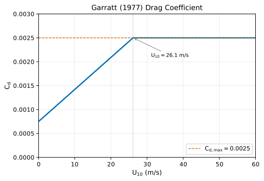
Fig. 25 Garratt (1977) drag coefficient showing linear growth capped at \(C_{d,\max} = 0.0025\). The transition occurs near 26 m/s.

Wind Stress Limiter

To prevent abrupt wind stress changes at the wet/dry boundary, Cocoa applies a depth-dependent limiter that smoothly ramps wind stress to zero as water depth approaches the drying threshold \(H_0\). This is always active and improves stability during wetting/drying cycles with strong winds.

The limiter computes a scaling factor \(f_w \in [0, 1]\):

(14)\[\begin{split}f_w(H) = \begin{cases} 1 & H > 4 H_0 \\[4pt] \dfrac{1}{2}\tanh\!\left(\dfrac{8\,(H - 2.5\,H_0)}{4\,H_0}\right) + \dfrac{1}{2} & H_0 < H \le 4 H_0 \end{cases}\end{split}\]

Since both GWCE and momentum kernels iterate only over wet nodes/elements (where \(H > H_0\) by construction), the \(H \le H_0\) case is never reached. The early return for \(H > 4 H_0\) avoids the tanh evaluation for the vast majority of the domain, where all threads in a GPU warp take the same branch with no divergence.

This formulation follows ADCIRC’s windLimiter subroutine (DMW 2022).

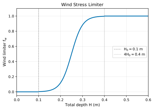
Fig. 26 Wind stress limiter \(f_w\) smoothly transitions from 0 near the drying threshold \(H_0\) to 1 at \(4H_0\), suppressing wind forcing in nearly-dry cells.

Application in the Momentum Equations

In the momentum equations ((2), (3)), wind stress appears as a surface forcing divided by the water column depth:

(15)\[F_x^{wind} = \frac{f_w \, \tau_{sx}/\rho_0}{H}, \quad F_y^{wind} = \frac{f_w \, \tau_{sy}/\rho_0}{H}\]

where \(\tau_s/\rho_0\) is the kinematic wind stress ((13)), \(H\) is the total water depth, and \(f_w\) is the wind stress limiter ((14)).

Discretized form (nodal):

Wind stress is applied per node after the element-based RHS assembly, with Crank-Nicolson centering between the two time levels:

\[RHS_{x,i} \mathrel{+}= \frac{\Delta t}{2} \, f_{w,i} \left( \frac{R_{met}^{n} \, \tau_{sx,i}^{n}/\rho_0}{H_i^{n}} + \frac{R_{met}^{n+1} \, \tau_{sx,i}^{n+1}/\rho_0}{H_i^{n+1}} \right)\]

and identically for \(RHS_{y,i}\), where \(R_{met}\) is the meteorological ramp factor (see Meteorological Ramp; the stress fields are stored pre-ramped) and \(f_{w,i}\) is evaluated at the \(n+1\) depth.

Application in the GWCE

In the GWCE ((6)), wind stress enters the \(\mathbf{J}\) vector as a depth-integrated surface forcing, scaled per node by the wind limiter before element averaging:

(16)\[J_x^{wind} = \frac{R_{met}}{3} \sum_{i=1}^{3} f_{w,i} \, \frac{\tau_{sx,i}}{\rho_0}, \quad J_y^{wind} = \frac{R_{met}}{3} \sum_{i=1}^{3} f_{w,i} \, \frac{\tau_{sy,i}}{\rho_0}\]

where \(f_{w,i}\) is the wind limiter evaluated at node \(i\) using that node’s total depth \(H_i = h_i + \zeta_i\). Unlike the momentum equation, wind stress in the GWCE is not divided by depth. The GWCE operates on depth-integrated quantities, and wind stress is a surface force per unit area.

Atmospheric Pressure Gradient

The atmospheric pressure gradient force accelerates water from high to low atmospheric pressure. This is the primary mechanism by which storm surge is generated, with the “inverted barometer” effect producing roughly 1 cm of surge per 1 hPa of pressure deficit.

Application in the GWCE

The atmospheric pressure gradient enters the GWCE through the \(\mathbf{J}\) vector:

(17)\[J_x^{atm} = -\frac{\alpha_L \, \bar{H}}{\rho_0 \cdot 2A_e} \sum_{i=1}^{3} p_{s,i} \cdot FDX_i, \quad J_y^{atm} = -\frac{\alpha_L \, \bar{H}}{\rho_0 \cdot 2A_e} \sum_{i=1}^{3} p_{s,i} \cdot FDY_i\]

where:

• \(p_{s,i}\) is the atmospheric pressure at node \(i\) [Pa]

• \(\alpha_L\) is the wet/dry slope limiter

• \(\bar{H}\) is the element-averaged total depth

• \(FDX_i, FDY_i\) are the shape function derivative products

The slope limiter \(\alpha_L\) is applied consistently with the tide potential gradient (see Generalized Wave Continuity Equation (GWCE)), reducing pressure gradients in shallow water to suppress spurious oscillations.

Pressure ramping:

During spinup, the atmospheric pressure is blended from the background reference pressure toward the actual forcing data:

(18)\[p_{s}^{ramped} = p_{bg} + R_{met} \cdot (p_s - p_{bg})\]

where \(p_{bg} = 101300\) Pa is the background atmospheric pressure and \(R_{met}\) is the meteorological ramp factor. This ensures a smooth transition from hydrostatic equilibrium at initialization.

Application in the Momentum Equations

In the momentum equations, the atmospheric pressure gradient appears alongside the barotropic pressure gradient:

\[F_x^{atm} = -\frac{1}{\rho_0}\frac{\partial p_s}{\partial x}, \quad F_y^{atm} = -\frac{1}{\rho_0}\frac{\partial p_s}{\partial y}\]

This term is already present in the momentum equation formulation (see (2)). For storm surge simulations, the atmospheric pressure gradient typically dominates over wind stress in deep water, while wind stress becomes more important in shallow coastal areas.

Meteorological Ramp

To prevent impulse responses at initialization, meteorological forcing is gradually introduced using a normalized hyperbolic tangent ramp function:

\[R_{met}(t) = \frac{1}{\tanh(2)}\tanh\left(\frac{2t}{T_{ramp}}\right)\]

where \(t\) is the elapsed time since cold start and \(T_{ramp}\) is the ramp duration. The normalization by \(\tanh(2)\) ensures the ramp reaches exactly 1.0 at \(t = T_{ramp}\), and the value is clamped to 1.0 for \(t \ge T_{ramp}\).

By default, the meteorological ramp uses the same configuration as the tidal ramp (forcing.ramp). An optional forcing.meteorological.ramp section allows a different ramp duration for meteorological forcing — useful when starting from a pre-spun-up tidal state that needs only a short met ramp. Internally, ForcingManager maintains separate ramp objects for tidal and meteorological forcing.

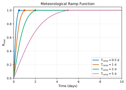
Fig. 27 Normalized hyperbolic tangent ramp for several \(T_{ramp}\) values. Dots mark \(t = T_{ramp}\) where \(R_{met} = 1.0\).

Temporal Interpolation

Meteorological forcing data is provided at discrete time snapshots. Between snapshots, Cocoa linearly interpolates the forcing fields:

\[\phi(t) = (1 - \alpha) \, \phi_{k} + \alpha \, \phi_{k+1}\]

where \(\alpha = (t - t_k) / (t_{k+1} - t_k)\) is the interpolation weight and \(\phi\) represents any forcing field (pressure, wind_u, wind_v).

The interpolation is performed at each mesh node after spatial interpolation from the meteorological grid. Cocoa maintains a ring buffer of pre-read snapshots to amortize I/O costs across timesteps.

Spatial Interpolation

Meteorological data is typically provided on a regular rectangular grid at coarser resolution than the computational mesh. Cocoa uses bilinear interpolation to transfer forcing data from the meteorological grid to mesh nodes.

For a mesh node located at \((x, y)\) within a grid cell with corners at \((x_0, y_0)\) and \((x_1, y_1)\):

(19)\[\phi(x, y) = w_{00} \, \phi_{00} + w_{10} \, \phi_{10} + w_{01} \, \phi_{01} + w_{11} \, \phi_{11}\]

where the bilinear weights \(w_{ij}\) are products of the normalized distances:

\[s = \frac{x - x_0}{x_1 - x_0}, \quad t = \frac{y - y_0}{y_1 - y_0}\]

\[w_{00} = (1-s)(1-t), \quad w_{10} = s(1-t), \quad w_{01} = (1-s)t, \quad w_{11} = st\]

The interpolation weights are precomputed once when the meteorological data is initialized and cached for reuse at each timestep. For regular (rectangular) grids, this is a simple index computation. For irregular grids (OWI NetCDF with moving vortex tracking), the weights are recomputed when the grid moves.

Multi-Domain Composition

Cocoa can compose several meteorological sources into one forcing field – each a forcing.meteorological.domains entry, of any format, or the flat single-source form – rather than being limited to one format per run. During interpolation, Cocoa applies a priority rule: the innermost valid domain takes precedence over outer domains, where “innermost” ranks first by configured source order (later entries win at overlap) and then, within a source that is itself multi-domain, by that source’s own domain index. Mesh nodes that fall outside all domains receive background values (101300 Pa pressure, zero wind). OWI’s internal nesting of several grids within one file (a coarse outer grid plus fine inner grids) is the same last-wins rule applied one level deeper, not a separate mechanism – composition is format-agnostic.

This approach allows, for example, a coarse basin-scale field to cover the full model domain while a fine hurricane-following nest – from the same source or a different one entirely (e.g. a GRIB regional model nested inside a coarser OWI field) – provides high-resolution forcing in the region of interest.

Cadence Interpolation onto the Union Time Axis

Composed sources need not share a common time step. Cocoa builds a single union time axis as the sorted, deduplicated set of every domain’s own sample times, and reads each domain against it. Where a union time coincides with one of a domain’s own samples, that domain’s data is used verbatim – exact, not interpolated. Where a union time falls strictly between two of a domain’s own samples (a coarser-cadence source relative to the axis), the domain’s fields – and, for a moving grid, its coordinates – are linearly interpolated between its own bracketing snapshots:

\[\phi_d(t) = (1 - \beta) \, \phi_{d,k} + \beta \, \phi_{d,k+1}, \qquad \beta = \frac{t - t_{d,k}}{t_{d,k+1} - t_{d,k}}\]

where \(\phi_d\) is domain \(d\)’s field, \(t_{d,k}\) and \(t_{d,k+1}\) are its own bracketing sample times, and \(t\) is the union-axis time being synthesized. This source-side (grid-space) interpolation is distinct from the node-side temporal blend of Temporal Interpolation: it lets a coarse-cadence source (e.g. a 3-hourly field) coexist with a fine-cadence one (e.g. hourly) on the same union axis without forcing every composed source to share a time step.

Activation Window Fade

A source active only over part of the run – a moving nest, or any source with a configured activation window – can be given an activation/deactivation cross-fade duration \(T\) (activation_ramp_seconds), applied at its window’s open and close times \(t_{open}\), \(t_{close}\) on the union axis:

\[w(t) = \text{tanh\_ramp}(t - t_{open},\, T) \cdot \text{tanh\_ramp}(t_{close} - t,\, T)\]

using the same normalized tanh shape as the cold-start meteorological ramp (Meteorological Ramp), but referenced to the source’s own window edges rather than to cold start. Where the source covers a node, the composed field cross-fades toward it, \(\text{node} = (1 - w) \cdot \text{underlying} + w \cdot \text{source}\), in place of the hard override of the priority rule above. \(T \le 0\) (the default) disables the fade, recovering hard window edges. The same weight gates the Eulerian per-domain combine, the Lagrangian moving-grid overlay, and the GAHM vortex overlay’s per-storm temporal factor, so a source – gridded or vortex – fades in and out identically regardless of which overlay mechanism carries it.

Wind Reduction

Cocoa optionally reduces wind velocity over land before applying the drag law. Two reduction mechanisms are supported, applied in sequence. Both are applied per meteorological source, folded into that source’s wind at composition time (before it is blended into the combined field), gated by the source’s wind_reduction flag. This lets co-located sources be treated differently – for example reducing a parametric vortex while leaving an already-surface GFS field unreduced. A source covered node produces the same stress as a post-blend reduction would; only feather rings between a reduced and an unreduced source differ.

Directional Roughness Reduction

The directional roughness reduction modifies wind components based on the ratio of upwind land surface roughness to marine roughness. This follows ADCIRC’s ApplyDirectionalWindReduction formulation.

Marine roughness is derived from the Garratt drag coefficient via Charnock’s relation:

\[z_{0m} = \frac{0.018}{g} \, C_d \, U_{10}^2\]

where \(C_d\) is the drag coefficient computed from the pre-reduction wind speed.

Land roughness \(z_{0l}\) is obtained by linear interpolation from the two nearest directional bins. The mesh stores 12 roughness lengths per node (one per 30-degree bin, starting from East and proceeding counter-clockwise).

Overland flooding correction: When the total water depth \(H = h + \zeta\) exceeds \(2 h_0\) (twice the minimum depth threshold), the effective land roughness is reduced:

\[z_{0l}^{eff} = z_{0l} - \frac{H}{30}\]

This accounts for the reduced influence of land surface features when they are submerged by floodwater.

Reduction factor: When \(z_{0l} > z_{0m}\), the wind reduction factor is:

\[f_r = \min\left(1,\; \left(\frac{z_{0l}}{z_{0m}}\right)^{0.0706} \frac{\ln(10 / z_{0l})}{\ln(10 / z_{0m})} \right)\]

When \(z_{0l} \le z_{0m}\) (land is smoother than open water), no reduction is applied (\(f_r = 1\)). The reduced wind components are:

\[u_{10}' = f_r \, u_{10}, \quad v_{10}' = f_r \, v_{10}\]

Canopy Coefficient

The canopy coefficient \(C_c \in \{0, 1\}\) is a binary multiplicative factor representing wind attenuation under forest canopy:

\[u_{10}'' = C_c \, u_{10}', \quad v_{10}'' = C_c \, v_{10}'\]

A value of \(C_c = 1\) (default) means no canopy effect; \(C_c = 0\) suppresses the wind (and hence the stress) at that node. The coefficient is folded into the source wind here rather than scaling the post-drag stress. For a binary mask this is exact – \(0\) and \(1\) are unchanged by the drag law’s squaring, so \(C_c = 0\) gives zero stress and \(C_c = 1\) is a no-op either way – which is why fractional values are rejected at startup. After both reductions the corrected source winds are blended, and the combined field is passed to the Garratt drag law ((12), (13)) once, after the meteorological ramp.

Physical Constants

Constant	Value	Description
\(\rho_0\) (seawater density)	1000 kg/m3	Reference density (ADCIRC convention)
\(\rho_a\) (air density)	1.293 kg/m3	Dry air density at 0 °C (ADCIRC convention)
\(p_{bg}\) (background pressure)	101300 Pa	Ambient pressure away from any storm (1013 mb, the ADCIRC/ATCF convention). The parametric vortex resolves its OWN far-field \(p_n\) per track snapshot from the ATCF RADP column and falls back to this value only when that column is blank; see Parametric Vortex (GAHM).
\(g\) (gravity)	9.81 m/s2	Gravitational acceleration
\(C_{d,\max}\) (drag cap)	0.0025	Default maximum drag coefficient

Implementation Files

• forcing/meteorological/DragLaw.hpp: wind_drag<DragLaw>() Garratt drag coefficient and wind_ice_drag<DragLaw, Attenuation>() ice attenuation (device-callable)

• forcing/meteorological/WindStress.hpp: wind_stress<DragLaw>() free function template for kinematic wind stress (device-callable)

• forcing/meteorological/WindReduction.hpp: Directional wind reduction kernel (device-callable)

• physics/WindLimiter.hpp: Depth-based wind stress limiter for drying cells (device-callable)

• numeric/terms/WindStressTerm.hpp: GwceWindStress wind stress GWCE contribution

• numeric/terms/AtmPressureGradient.hpp: GwceAtmPressureGradient atmospheric pressure gradient GWCE contribution

• numeric/momentum/MomentumRhsKernels.cpp: Wind stress in momentum RHS

• forcing/meteorological/MeteoForcingProvider.hpp: Ring buffer, temporal interpolation, and overlay orchestration

• forcing/meteorological/MeteoSnapshotSource.hpp: Rank-0 reader thread; union time axis, per-domain windows, cadence interpolation

• cocoa_meteo/CompositeMeteoReader.hpp: Composes multiple configured sources into one flat, priority-ordered domain space

• cocoa_meteo/interpolation/MultiDomainInterpolator.hpp: Host spatial combine, priority rule, winner mask, activation weights

• forcing/WindowedRamp.hpp: Activation/deactivation window fade (shared tanh shape with Ramp)

• forcing/ForcingManager.hpp: Ramp computation, wind reduction, and forcing orchestration