Baroclinic Coupling

Cocoa can couple a depth-averaged (2DDI) hydrodynamic solve to an external 3D ocean climatology through three terms: a horizontal baroclinic pressure gradient (BPG) with its free-surface correction, an internal-tide wave-drag friction enhancement, and a dispersion friction correction. All three read a single preprocessor-generated nodal forcing file (Configuration) and share a common activation ramp.

The method follows the 2DDI approach of Pringle et al. (2019) [Pringle2019] and its global application [Pringle2021], as refined in ADCIRC by C. Blakely, whose global tidal dissipation analysis [Blakely2022] underpins the internal-tide drag’s role in the global model. The internal-tide and dispersion terms are carried over from ADCIRC’s nodalattr.F and internaltide.F90.

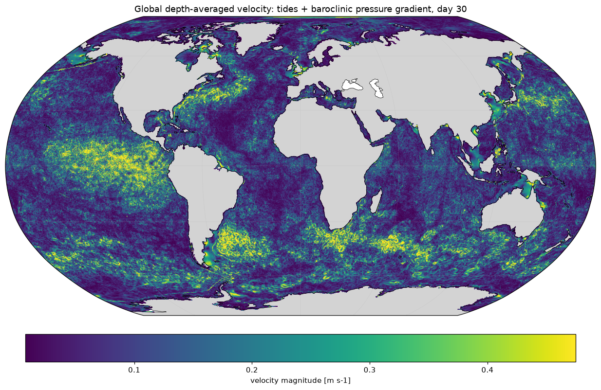
Global depth-averaged velocity after 30 days of tidal plus baroclinic forcing — Fig. 6 Depth-averaged velocity magnitude on a 3.7M-node global shell, forced by tides plus a single frozen (diagnostic-mode) RTOFS density snapshot, at day 30 of spin-up. The western boundary currents and the Antarctic Circumpolar Current are resolved.

Overview 

A depth-averaged model has no vertical structure, so it cannot represent the pressure gradient a real 3D density field produces, the drag a stratified ocean exerts on the barotropic tide through internal-wave generation, or the extra bottom friction implied by unresolved vertical shear. Cocoa closes these gaps with fields computed offline from a 3D ocean climatology (HYCOM GOFS 3.1) by the cocoa_ocean3d Python preprocessor and interpolated onto mesh nodes as a CF NetCDF time series:

BPG + free-surface correction (Baroclinic pressure gradient): enters GWCE and momentum as an extra pressure-gradient forcing, exactly like the barotropic term.
Internal-tide wave drag (Internal-tide wave drag): an additional symmetric 2x2 friction-tensor contribution, active only where internal tides can propagate freely.
Dispersion as friction (Dispersion as friction): a further friction-tensor contribution representing depth-averaging error.

All three are gated independently under forcing.baroclinic (see Configuration) and share the file’s BPG, sigma-t, buoyancy-frequency, and mixed-layer products; enabling internal-tide drag or dispersion without the parent enabled: true is rejected at startup.

Theory 

Baroclinic pressure gradient 

The 2DDI BPG at a mesh node is a depth-averaged, horizontal derivative of the baroclinic pressure anomaly

\[\mathrm{BPG}_x = \frac{g}{\rho_0 H}\int_{-H}^{0} \int_{-H}^{z}\frac{\partial \rho}{\partial x}\,dz'\,dz,\]

computed by the preprocessor from a TEOS-10 (GSW) in-situ density profile via one-sided horizontal differences and a trapezoidal vertical integral (cocoa_ocean3d.bpg). \(\mathrm{BPG}_y\) is defined identically in the meridional direction. Both are staggered, with BPGX at longitude midpoints and BPGY at latitude midpoints, and the vertical integral is truncated at the shallower of any two neighboring wet columns, never extrapolated past the shallower column’s seabed. The preprocessor clamps the horizontal density-anomaly bracket to \(\pm 0.1\) kg/m ³ before scaling by \(g/\rho_0\), bounding \(|\mathrm{BPG}| \le g/\rho_0 \times 0.1 \approx 9.8\times10^{-4}\) m/s ².

The BPG enters GWCE and momentum with the same sign convention as the barotropic pressure gradient (Physics::BaroclinicGradient::compute_momentum_contribution / compute_gwce_contribution): the momentum contribution is area-weighted and Crank-Nicolson time-centered,

\[\Delta(\text{momentum RHS}) = -\frac{\Delta t}{2}\, A_e\, \bigl(\overline{\mathrm{BPG}}^{\,n} + \overline{\mathrm{BPG}}^{\,n+1}\bigr),\]

where \(\overline{\cdot}\) is the element’s 3-node average, and the GWCE contribution is the negative depth-weighted nodal average \(-\overline{H_i\,\mathrm{BPG}_i}\). Time-centering the BPG matches Cocoa’s other forcing terms (atmospheric pressure, tide potential, wind stress); the nodal reader already brackets two snapshots, so time-centering costs nothing and keeps the RHS assembly internally consistent.

Free-surface correction 

The BPG above is computed from a fixed reference density profile and does not know the model’s own free surface. Pringle et al. [Pringle2019] correct for this by adding the elemental gradient of the surface potential-density anomaly (sigma-t) times the live free-surface elevation,

\[\Delta\mathrm{BPG}_{\mathrm{FS}} = \frac{g}{\rho_0}\, \nabla\bigl(\sigma_t\,\eta\bigr),\]

evaluated with the linear-basis element gradient coefficients already resident for the pressure-gradient term (MomentumRhsKernels.cpp’s spatial_grad_a/b). The term is recomputed every step from the current eta and the time-interpolated sigma_t and added into the effective bpg_x/bpg_y fields before either consumer reads them, so the momentum and GWCE contributions both include it. A node whose surface sigma-t is the missing-value sentinel (see Nodal forcing file) zeroes the whole element’s correction.

Internal-tide wave drag 

A barotropic tide flowing over rough topography in a stratified ocean radiates internal waves, extracting momentum from the barotropic flow. Cocoa represents this as an additional symmetric 2x2 contribution to the friction tensor (Momentum Equations), driven by a user-supplied topographic nodal attribute and the file’s runtime bottom/mean buoyancy frequencies (\(N_b\), \(N_m\)). Three forms are supported, selected by the attribute’s column count (physics.internal_tide_friction: mesh, an existing NodalAttributeReader variable named internal_tide_friction):

Nycander (2005) [Nycander2005], 5-column (“nonlocal”): columns are the coefficient \(C\) and two topographic-slope pairs \((H_x, H_y)\), \((J_x, J_y)\),

\[\mathrm{Fit} = C\,\frac{N_b}{H}\sqrt{1 - f^2/\omega^2}, \qquad \gamma^2 = \frac{H_x^2 + H_y^2}{(\omega^2-f^2)/(N_b^2-\omega^2)}, \qquad \mathrm{Fit} \leftarrow \frac{\mathrm{Fit}}{\max(1,\gamma^2)},\]

with tensor add \((2\,\mathrm{Fit}\,H_xJ_x,\ 2\,\mathrm{Fit}\,H_yJ_y,\ \mathrm{Fit}(H_xJ_y+H_yJ_x))\) for \((xx, yy, xy)\).
Lyard et al. (2004) [Lyard2004], 3-column (“local”) and its Zaron & Egbert (2006) [ZaronEgbert2006] 2-column scalar form share one drag coefficient,

\[\mathrm{Fit} = C\,\frac{\sqrt{(N_b^2-\omega^2)(N_m^2-\omega^2)}}{\omega} \Big/ \max\Bigl(1,\ \frac{\omega^2-f^2}{N_b^2-\omega^2}\Bigr),\]

isotropic (\(C_{xx}=C_{yy}=\mathrm{Fit}\cdot\text{slope}^2\), \(C_{xy}=0\)) for the scalar form, or the full tensor (\(C_{xx}=\mathrm{Fit}H_x^2\), etc.) for the 3-column form.

Both forms act only where internal tides can propagate freely: \(\omega < N_b\) (supercritical stratification) and \(\omega > |f|\) (above the local inertial frequency), \(\omega\) being the M2 tidal frequency (Constants::omega_m2(), \(1.4052\times10^{-4}\) rad/s) throughout. Outside those bounds the tensor add is exactly zero. A 1/3-column attribute without baroclinic coupling (forcing.baroclinic.internal_tide.enabled: false) is the static form: the raw attribute values are added to the friction tensor directly, with no \(N_b\)/\(N_m\)/de-tiding dependence; a 5-column attribute always requires the coupling (there is no static Nycander equivalent) and is rejected at startup otherwise.

Two conventions differ from the published formulation so that an ADCIRC fort.13 converted by utils/cocoa_mesh_tools.py keeps working with the values it already has.

First, the coefficient: [Pringle2019] (Eq. 5) writes the drag tensor with a \(4\pi\) in the denominator and reports a tuned \(C_{it} = 4.0\). Neither ADCIRC nor Cocoa carries the \(4\pi\); both fold it into the attribute value, so the number in column 1 is \(C_{it}/4\pi\) (about 0.318 for the paper’s 4.0), and taking \(C_{it}\) straight from the paper overstates the drag by a factor of about 12.6.

Second, the shelf cutoff: [Pringle2019] sets \(\mathcal{C} = 0\) where \(h < 100\) m to prevent excessive dissipation on the continental shelves, while Cocoa applies no such depth gate (the only cutoffs are the propagation bounds above). internal_tide_friction is a user-supplied mesh attribute that cocoa_ocean3d does not generate, so zeroing it on the shelf is the responsibility of whatever produced the attribute. An ADCIRC fort.13 prepared for the published method already carries that zeroing; an attribute built from raw topographic slopes does not, and will dissipate energy across the shelf.

De-tiding 

The internal-tide and dispersion formulas above act on the non-tidal (subtidal) velocity, not the raw depth-averaged velocity, which is dominated by the barotropic tide itself. Cocoa extracts the non-tidal component with a 25-hour, 12-minute-sampled lagged boxcar mean (equivalent to ADCIRC’s UNTIDE, including its partial mean during the first 25 hours of spin-up), then forms a capped de-tiding ratio

\[\mathrm{adju} = \min\!\Bigl(\frac{D_{\mathrm{tidal}}}{D_{\mathrm{total}}},\ 100\Bigr), \qquad D = C_{xx}u^2 + 2C_{xy}uv + C_{yy}v^2\ \text{(evaluated at raw and de-tided velocity)},\]

that scales the internal-tide tensor contribution: a steady (non-tidal) flow has \(D_{\mathrm{tidal}}=0\), so the drag reduces to bare friction, while a pure oscillation has the de-tided velocity go to zero, so \(\mathrm{adju}\to1\). The ring state and the effective BPG pair are persisted, so a mid-window restart reproduces an uninterrupted run exactly (see Checkpoint format).

The ring buffer’s sampling is entirely device-resident: float ring samples and double running accumulators (~1.6 GB and 25.6 MB at 1.6M nodes). The window-crossing decision (whether this step is the ~1-in-360 step that samples) is made on the host from a mirror of the last-sample time, so the per-node sampling kernel launches only on crossing steps and no per-step scalar deep_copy fence exists on either path.

Dispersion as friction 

Depth averaging discards a vertical shear dispersion term. Cocoa adds a further diagonal friction-tensor contribution, active only in deep water (dispersion.deep_water_depth, default 1000 m, tested against the local bathymetric depth rather than total depth so the gate does not chatter with the tide):

\[\mathrm{add}_{xx} = \mathrm{ramp}\cdot c_d\cdot \mathrm{adj}_u\cdot \frac{\lVert(\bar u,\bar v)\rVert}{H}, \qquad \mathrm{add}_{yy} = \mathrm{ramp}\cdot c_d\cdot \mathrm{adj}_v\cdot \frac{\lVert(\bar u,\bar v)\rVert}{H},\]

with \(\mathrm{adj}_u,\mathrm{adj}_v\) the same capped de-tiding ratio form as above, under a symmetric \([-100,100]\) cap since this ratio, unlike the internal-tide ratio, is a raw mean-over-instantaneous quotient that can be negative during a tidal reversal. Both ratios are applied under a single joint \(|u|,|v|>10^{-3}\) guard: a large \(u\) with a near-zero \(v\) still gets \(\mathrm{adj}_u=1\), not the ratio. The off-diagonal entry is never touched by this term. \(c_d\) comes from one of two modes (dispersion.mode):

mld (mixed-layer-depth power law): \(c_d = a\,(x^b - 1)\), where \(x\) is the file’s dimensionless mixed_layer_ratio, floored at \(4\times10^{-3}\) before the power. a/b are required config keys with no default; appropriate values are case-specific.
cdisp (direct coefficient): \(c_d\) is the file’s dispersion_cd value directly, clamped to \(\le 1.0\) at read time.

mixed_layer_ratio is the mixed-layer depth divided by the local wet depth and is at most 1 by construction (see Nodal forcing file), so with positive a and b the power law gives \(c_d \le 0\) and the term reduces friction. The positive-semidefinite clamp below keeps the combined tensor physical when this reduction, together with a tidal-reversal sign flip in \(\mathrm{adj}_u\)/\(\mathrm{adj}_v\), would otherwise drive a diagonal entry negative.

Positive-semidefinite clamp 

Internal-tide drag and dispersion are both added on top of the base Manning-friction tensor; either can, in principle, push the combined symmetric 2x2 tensor non-positive-semidefinite, an unphysical friction that would inject energy. Cocoa applies a closed-form eigenvalue floor (physics/FrictionTensorPsd.hpp) after every additive contribution:

\[\lambda_{1,2} = \frac{\mathrm{tr}}{2} \pm \sqrt{\left(\frac{xx-yy}{2}\right)^2 + xy^2},\]

with any negative eigenvalue floored at zero and the tensor reconstructed from the unchanged eigenvectors. The clamp is an exact no-op on the pure Manning tensor (\(xy=0\) makes both eigenvalues equal the non-negative diagonal entries), so the path with no internal tide and no dispersion reproduces Cocoa’s pre-baroclinic references exactly, a standing regression test.

Preprocessor pipeline 

The cocoa_ocean3d Python package (utils/cocoa_ocean3d) produces the nodal forcing file in three stages tied together by pipeline.SnapshotRegridder:

Compute (compute.compute_snapshot): TEOS-10 (via the gsw package) in-situ density from practical salinity and in-situ temperature, using gsw.p_from_z for the depth-to-pressure conversion. BPGX/BPGY, surface sigma-t, \(N_b\)/\(N_m\) (bottom and depth-mean buoyancy frequency via gsw.Nsquared), and the mixed-layer ratio (a de Boyer Montegut et al. 2004 [DeBoyerMontegut2004] fixed 0.03 kg/m³ sigma-t-anomaly criterion) are all computed here.
Regrid (regrid.compute_weights/apply_weights): bilinear by default, falling back to a box average when the mesh’s local neighboring-element-centroid footprint spans more source grid cells than a configurable threshold. A fill guard (any contributing source cell non-finite) NaNs the regridded node value.
Write (writer.NodalForcingWriter): the CF nodal file (see Nodal forcing file), one call per snapshot, append-safe (an existing file’s time axis is validated and extended, never silently overwritten).

The cocoa-ocean3d CLI wraps download/compute/regrid/all subcommands against HYCOM GOFS 3.1 (experiment IDs isolated in a module-level table). No live-network tests run in CI; download logic is tested against recorded fixtures.

Configuration 

Key	Default	Description
`forcing.baroclinic.enabled`	`false`	Master switch. There is no scalar-constant fallback: the nodal file is either present and read, or the feature is off entirely.
`forcing.baroclinic.filename`	(required if enabled)	Nodal forcing NetCDF path (see Nodal forcing file).
`forcing.baroclinic.ramp`	enabled, `1d`	One-sided cold-start spinup ramp (normalized tanh, 0 at `simulation.start_time` rising to 1 over `duration`), shared by the BPG/free-surface correction, the dynamic internal-tide drag, and dispersion, so `ramp_factor == 0` reproduces the pre-baroclinic friction tensor exactly. Independent of the global `forcing.ramp` (disabling one does not disable the other). A static `internal_tide_friction` attribute is not a baroclinic contribution (it is legal with no baroclinic file at all), so it is left unramped.
`forcing.baroclinic.internal_tide.enabled`	`false`	Activates the dynamic (\(N_b\)/\(N_m\)-driven) internal-tide drag. Requires `physics.internal_tide_friction: mesh` naming a 2/3/ 5-column `internal_tide_friction` nodal attribute. Gated separately from the BPG, but still requires the parent `enabled: true` (the shared file supplies \(N_b\)/\(N_m\)).
`forcing.baroclinic.dispersion.enabled`	`false`	Activates dispersion-as-friction. Requires `internal_tide.enabled: true` (dispersion rides on the same de-tided `adju`/`adjv` machinery internal-tide drag needs).
`forcing.baroclinic.dispersion.mode`	`mld`	`mld` or `cdisp`; see Dispersion as friction.
`forcing.baroclinic.dispersion.deep_water_depth`	`1000.0` [m]	Deep-water gate on local bathymetric depth.
`forcing.baroclinic.dispersion.mld_coefficients.a`/`b`	(required if mode: mld)	Power-law coefficients applied to the dimensionless `mixed_layer_ratio`; no default exists, and appropriate values are case-specific. Any positive pair produces \(c_d \le 0\) (see Dispersion as friction).

forcing:
  baroclinic:
    enabled: true
    filename: "baroclinic_forcing.nc"
    ramp:
      enabled: true
      duration: 12h
    internal_tide:
      enabled: true
    dispersion:
      enabled: true
      mode: mld
      deep_water_depth: 1000.0
      mld_coefficients:
        a: 0.01
        b: 0.5
  tide:
    # ... tidal forcing, unaffected by baroclinic coupling ...

physics:
  internal_tide_friction: mesh   # required when internal_tide.enabled

Nodal forcing file 

CF-1.8 NetCDF, dims (time, node), written by the preprocessor and read by a reader modeled on FlowTimeSeries’s snapshot-bracketing shape (distributed owned+ghost read, linear time interpolation, persistent device Views allocated once).

Variable	Units	Required when
`time`	CF numeric (seconds since an epoch the file itself declares)	always
`bpg_x`, `bpg_y`	m s^-2	always
`sigma_t_surface`	kg m^-3	always
`n_bottom`, `n_mean`	s^-1	`internal_tide.enabled`
`mixed_layer_ratio`	1 (dimensionless)	`dispersion.enabled` and `mode: mld`
`dispersion_cd`	1 (dimensionless)	`dispersion.enabled` and `mode: cdisp`

One file covers every product; the conditional variables above let a run enable any subset without forking the file format. A frozen file (exactly one time value) applies for the whole simulation window (diagnostic mode) and is exempt from the reader’s time-coverage validation.

Missing-value convention (binding on both the writer and the reader): every variable declares _FillValue = NaN, but only sigma_t_surface may legally carry it in a well-formed file. The preprocessor zero-fills BPG/N/dispersion products at dry columns (so a coastal bilinear blend fades toward zero forcing), while surface sigma-t is NaN at any node whose regridding stencil touches a dry/land source cell. NaN in any other variable is a fail-loud file error naming the variable and the first offending node; the free-surface-correction kernel is the one consumer of the sigma_t_surface NaN sentinel (see Free-surface correction).

Global attributes: Conventions (“CF-1.8”), title/institution/ source/history (CF provenance), mesh_num_nodes (validated against the reader’s own count, fail loud on mismatch), mesh_id (the cm1P.. fingerprint, when the writer could compute one; validated when present, not required), source_dataset, utility_version, generation_command.

The file stores every product in fp64. In the model the nodal fields are narrowed to float (Types::promote/Types::narrow at the read/write boundary, the same convention the friction and lateral-stress tensors use); all arithmetic on them stays double, including the free-surface-correction accumulation, which keeps a dedicated fp64 scratch pair. Float storage sits below the information content of the source data (an OGCM analysis differentiated onto the mesh carries four to five significant digits), and the momentum element kernel’s per-node gather of the Crank-Nicolson pair was the single largest per-step cost the coupling added. The same kernel reads that pair pre-summed (the compose pass forms bpg_effective_*_prev + bpg_effective_* in the node sweep it already runs), so momentum gathers two nodal arrays rather than four.

Regression checks 

Every layer pins a “zeros reproduce the pre-baroclinic baseline” invariant: an all-zero nodal forcing file with baroclinic enabled must reproduce the same-config baroclinic-disabled run exactly (Integration_WNAT_baroclinic_zero_forcing), a static internal-tide attribute of zeros must reproduce baseline, and a disabled dispersion path must reproduce baseline. These checks prove the gating is correct independent of the physics itself. The composed integration test (Integration_WNAT_baroclinic_composed) runs the opposite direction: with the BPG, free-surface correction, internal-tide drag, and dispersion all active, the run must differ measurably from its baroclinic-disabled counterpart, backed by a committed reference at the same 1e-6 cross-run tolerance used by the other WNAT implicit references.

Checkpoint format 

The internal-tide de-tiding ring buffer’s state (ring samples as float with two velocity components, the double running accumulator, the ring write position, whether the buffer has completed a full cycle, and the last-sample simulation time) is persisted in Cocoa’s checkpoint format (Checkpoint / Restart), gated behind internal_tide.enabled like the existing meteorological/tide-potential state. The effective BPG pair and its previous level are likewise persisted (GWCE consumes the value composed during the previous step and momentum centers against the step before that, so both are live state carried across a step boundary), gated behind the baroclinic runtime state, and stay f8 on disk regardless of the in-model float storage. Both are additive checkpoint format changes (version 4); a checkpoint from a run without the corresponding forcing carries none of these fields. With every carried level in the file, a mid-window restart reproduces an uninterrupted run exactly.

Full citations are collected in References.