Global Simulations

Global ocean simulations raise two problems regional coastal models do not: coordinate singularities at the poles, and elements that cross the prime meridian or date line.

Overview

Unlike regional models that can ignore edge effects, global models must handle:

Pole singularities: The shallow water equations have singularities at the geographic poles, where meridians converge and the metric term \(\tan\phi / R_e\) diverges.
Meridian discontinuities: Elements that span the \(\pm 180\)° longitude line have coordinate discontinuities that can cause incorrect geometry calculations.
Spherical geometry: Scale factors and metric corrections become more important when the domain spans large latitude ranges.

Cocoa addresses these challenges through:

Automatic meridian crossing detection: Elements straddling the antimeridian are automatically detected and corrected during mesh initialization.
Coordinate rotation: An optional coordinate transformation that relocates the computational poles away from the geographic poles.

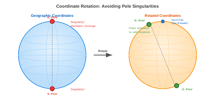
Coordinate rotation moves pole singularities away from geographic poles — Fig. 7 Coordinate rotation relocates the computational poles (singularities) from the geographic poles to other positions, usually well over land, effectively removing the singularities from the model.

When to Use Coordinate Rotation

Coordinate rotation is required when your global mesh includes elements near the geographic poles (typically within 5-10 degrees of \(\pm 90\)° latitude). Without rotation, simulations will experience:

Numerical instability from near-singular metric terms
Time step restrictions due to converging meridians
Degraded solution quality in polar regions

Coordinate rotation is not required for:

Regional models (any latitude range)
Global models that exclude polar regions (e.g., \(\pm 80\)° latitude bounds)

Configuration

Basic Global Mesh Setup

A minimal configuration for a global simulation without rotation:

mesh:
  filename: "global_mesh.nc"
  projection:
    type: "Mercator"
    center: [0.0, 0.0]  # Centered on equator

simulation:
  start_time: 2025-01-01
  end_time: 2025-02-01
  time_step: 60s  # Global models often need larger time steps

physics:
  manning_n: 0.025
  tau0: 0.005

The projection center [0.0, 0.0] places the reference point at the intersection of the prime meridian and equator, which is typical for global models.

Global Mesh with Coordinate Rotation

For global models including polar regions, enable coordinate rotation:

mesh:
  filename: "global_mesh_with_poles.nc"
  projection:
    type: "Mercator"
    center: [0.0, 0.0]
  rotation:
    enabled: true
    pole_location: [0.0, 0.0]  # New pole at (lon=0, lat=0)

The pole_location specifies where the geographic North Pole is relocated in the rotated coordinate system. This uses the same format as ADCIRC’s znorth_in_spherical_coors in the fort.rotm file.

Common choices:

Pole Location	Effect
`[0.0, 0.0]`	North Pole moves to equator at prime meridian
`[180.0, 0.0]`	North Pole moves to equator at date line
`[-90.0, 0.0]`	North Pole moves to equator in Atlantic

Choosing a Pole Location

When selecting the pole location, consider:

Avoid areas of interest: The new poles carry the numerical singularities, so place them where solution accuracy is less critical: over land, or in deep ocean far from your study area.
Land placement: Placing poles over land (e.g., Antarctica or northern Canada) is ideal if your mesh excludes those regions.
Match existing meshes: If your mesh was generated with ADCIRC’s rotated pole system (IFSPROTS=1), use the same pole location in Cocoa.

Understanding Rotation Effects

When coordinate rotation is enabled, several quantities are affected:

Coordinates

All node coordinates are transformed from geographic \((\lambda, \phi)\) to rotated \((\lambda', \phi')\) coordinates. The mesh file remains unchanged; transformations happen at runtime.

Coriolis Parameter

The Coriolis parameter \(f = 2\Omega\sin\phi\) uses the geographic latitude \(\phi\), not the rotated latitude \(\phi'\). The Coriolis effect depends on the component of Earth’s rotation vector along the local vertical, and rotating the coordinate system does not move either one: the rotation matrix \(R\) is orthonormal, so the rotated pole direction \(R\hat{z}\) and the rotated local vertical \(R\hat{r}\) have the same dot product as \(\hat{z}\) and \(\hat{r}\) did, namely \(\sin\phi\). Cocoa evaluates the rotated-frame form \(f = 2\Omega\,(R\hat{z})\cdot\hat{r}'\) on rotated meshes, which is the same number to machine precision.

Metric terms are the opposite case. The spherical correction \(\tan\phi/R_e\) and the projection scale factors are properties of the coordinate system the equations are discretized in, so they use the rotated latitude \(\phi'\). Keeping the two straight matters: the metric term is what would otherwise become singular at the pole, and pole rotation removes that singularity only if the term is evaluated in the rotated frame.

Tidal Potential

Tidal potential forcing (gravitational attraction from the Moon and Sun) uses geographic latitude \(\phi\). This is a physical requirement because the tidal potential depends on the actual position relative to celestial bodies.

Velocities

Velocities are computed in the rotated coordinate frame (rotated east/north directions). For output, Cocoa transforms velocities back to the geographic frame so that output files show true eastward (u) and northward (v) components.

Projection Selection

For global simulations, projection choice affects numerical accuracy:

Projection	Recommendation
Mercator	Best for global models with rotation. Conformal (angle-preserving) properties are important for accurate velocity calculations. Requires rotation if including high latitudes.
Equidistant Cylindrical	Acceptable for global models. Simple but introduces errors at high latitudes.
Equal Area	Good for mass conservation, but distorts shapes. Use when accurate integrated quantities are more important than local accuracy.
Miller	A compromise between Mercator and cylindrical equal-area. Moderate distortion at all latitudes.
Gall Stereographic	Cylindrical projection with two standard parallels at 45 degrees. Moderate distortion compromise.

Complete Example

A complete configuration for a global ocean model with tidal potential forcing, self-attraction and loading (SAL), and spatially varying friction. This corresponds to the Global Ocean test case:

output:
  step_interval: 5

diagnostics:
  screen_interval: 60
  log_file: log.json

mesh:
  filename: "global.nc"
  projection:
    type: "Mercator"
    center: [0.0, 45.0]
  rotation:
    enabled: true
    pole_location: [114.16991, 0.77432]

simulation:
  start_time: 2025-01-01
  end_time: 2025-02-01
  time_step: 12m

physics:
  manning_n: "mesh"
  cf_lower_limit: 0.0010
  tau0: 0.0022222
  smagorinsky_coefficient: 0.2
  min_viscosity: 1.0e-6

numeric:
  solver: implicit
  gwce_coefficients: [0.5, 0.5, 0.0]

forcing:
  ramp:
    enabled: true
    duration: 5d
  tide:
    sal:
      enabled: true
    potential:
      enabled: true

initial_conditions:
  water_level: 0.0

Key aspects of this configuration:

Coordinate rotation relocates the North Pole to [114.16991, 0.77432], placing the singularity over land (Borneo).
Mercator projection centered at 45°N provides conformal mapping.
Spatially varying friction (manning_n: "mesh") reads Manning’s n values from a mesh variable rather than using a uniform value.
SAL correction (tide.sal.enabled: true) accounts for self-attraction and loading effects on the tide.
Tide potential is enabled without specifying constituents — Cocoa automatically computes tidal potential forcing from built-in constituent parameters.
Implicit solver with gwce_coefficients: [0.5, 0.5, 0.0] enables the large 720-second time step needed for efficiency on a global domain.
No tidal boundary section is needed because a global mesh has no open boundaries.