Spectral Wave Model
Cocoa’s internal wave model is a third-generation spectral model that runs on the circulation mesh and exists to supply the wave force behind wave setup (Wave Forcing). Its physics is SWAN’s: the source terms are SWAN’s formulas (Source Terms) and its outputs are defined as SWAN writes them, so a Cocoa run can be set beside an ADCIRC+SWAN run [Dietrich2011] term for term. Its numerics are not SWAN’s. They were designed for GPUs from the properties of the discrete equations, and Where the Ideas Came From records which ideas came from SWAN, which from WAVEWATCH III and the wider literature, and which were worked out for Cocoa.
Governing Equation
The model evolves the action density \(N(\mathbf{x}, \sigma, \theta, t)\), the energy density over the intrinsic radian frequency, \(N = E/\sigma\), which is conserved in the presence of currents where energy is not [Booij1999]:
\(\hat{\boldsymbol\theta} = (\cos\theta, \sin\theta)\) is the direction the waves travel toward, counterclockwise from east, \(\mathbf{U}\) the depth-averaged current and \(c_g\) the group velocity from linear dispersion, \(\sigma^2 = gk\tanh kd\), which Cocoa solves exactly (SWAN uses Hunt’s approximation). The depth \(d = h + \eta\) and the current are the circulation’s at the coupling time, node by node, with no interpolation between meshes.
With \(\hat{\mathbf s} = \hat{\boldsymbol\theta}\) along the wave and \(\hat{\mathbf m} = (-\sin\theta, \cos\theta)\) across it, the speeds in spectral space are SWAN’s [Booij1999]:
The first term of \(c_\theta\) is depth refraction, written with the
wavenumber gradient at each frequency (SWAN’s default, WNUM); the second
is refraction by current shear; the third turns the waves along great
circles on the sphere, with \(\phi\) the latitude and \(R\) the
Earth’s radius. \(c_\sigma\) shifts frequency where the depth changes in
time or along the current, and where the current is strained. Gradients are
physical and taken in the circulation’s solver frame, so on a rotated-pole
mesh the great-circle term uses the rotated latitude and the poles never
appear.
The total source \(S_{tot}\), a rate of change of action density as every term below is written, sums wind input, quadruplet interactions, whitecapping, depth-induced breaking and bottom friction (Source Terms):
The Spectral Grid
Directions sit at the centers of equal cells around the circle, as SWAN places them. Frequencies are geometric from \(f_0\) to \(f_{max}\), with ratio \(r\) between neighbors, and each frequency owns the cell between its geometric midpoints, so the cells tile the range:
SWAN integrates with \(\sigma_f\ln r\) instead, 0.04 % narrower at \(r = 1.1\); the finite-volume width (48) is the one the frequency-shift flux balance needs. The finite-volume weight \(\sigma_f\Delta\sigma_f\Delta\theta\) weights the outer iteration’s convergence test (Solving a Step), the published parameters and the radiation stress; SWAN’s \(\sigma_f\ln r\,\Delta\theta\) weights the source terms’ integral parameters. Both are rules of the grid. The frequencies, their widths, the convergence test’s weights and the direction monomials are cached in tables built once per run, each on the side (device or host) that would otherwise evaluate it, so the cache returns the same bits. The defaults are the SWAN+ADCIRC hurricane grid: 36 directions and 41 frequencies from 0.031384 to 1.420416 Hz (\(r = 1.1\)). Choosing another grid is covered in Wave Forcing.
Transport Discretization
Median-Dual Finite Volumes
Each node owns the median-dual cell around it: every element contributes, at each of its vertices, the polygon from the vertex to the midpoints of its two edges and the element center (the centroid of a triangle, the vertex mean of a quadrilateral). The pieces tile the mesh, triangles and quadrilaterals alike. Two nodes that share an element edge share a dual face, the segment from the edge midpoint to the element center, with an integrated normal \(\mathbf n_{ij}\). Areas and normals are computed in the solver frame’s projection and divided by the map factors, so fluxes and volumes are physical on the sphere, with the same metric the circulation uses.
The face flux splits the advecting velocity \(\mathbf c = c_g \hat{\boldsymbol\theta} + \mathbf U\) at each node (flux-vector splitting), and a step of length \(\Delta t\) is backward Euler. For one bin at node \(i\) with dual volume \(V_i\):
with \(x^+ = \max(x,0)\), \(x^- = \min(x,0)\), \(B_i\) the step’s start (\(N^n\), plus the source terms folded into it, Solving a Step) and \(D_i\) everything on the diagonal: the outflow rates to the neighboring bins in direction and frequency, and the dissipation rates,
The spectral inflow is upwind by the sign of the neighboring bins’ speeds.
In frequency, upwinding alone spreads a shifting spectrum over its neighbors, an error first order in the bin width: on SWAN’s 10 % grid, an opposing current that shifts a wave 1.3 bins raised its mean frequency 5 % (Opposing Current). The frequency flux therefore carries a second-order MUSCL correction with van Leer’s monotonized-central limiter [vanLeer1977], formed in \(\ln\sigma\), where the geometric grid is uniform, on the action per unit \(\ln\sigma\), \(n = \sigma N\). Through the face between a bin \(u\) and its downwind neighbor \(d\), with \(uu\) the bin beyond \(u\):
The first term is the upwind flux in the matrix. The correction is
deferred: it is formed from the lagged spectrum, as the spectral inflow is,
and so holds exactly once the outer iteration has converged. The two bins of
a face compute the same correction, so action stays conserved. The limiter
zeroes the correction at a spectral peak; it is also zero between bins whose
speeds disagree in sign and at a face whose \(uu\) lies beyond the grid.
SWAN instead blends central and upwind differences (its CSS, 0.5), which
is comparably accurate but not positivity preserving. The correction adds
5 % to the wave model’s time on the full CPRA mesh and changes the Katrina
comparison with ADCIRC+SWAN by less than 1 % (Verification).
Every column of this matrix is diagonally dominant, with margin \(V_j/\Delta t\), because what leaves a cell enters a neighbor or leaves the domain. It is therefore an M-matrix, whose inverse is non-negative: the step conserves action and keeps it non-negative for any time step, on any mix of triangles and quadrilaterals [Varga2000]. That is what allows one step per coupling interval (600 s) on a coastal mesh whose Courant numbers run into the hundreds. The frequency correction sits on the right-hand side; while the iteration converges it can drive a row below zero, and that row is clipped to zero.
Median-dual finite volumes are not the residual-distribution N-scheme of WAVEWATCH III’s and WWM’s implicit unstructured solvers [Roland2012] [Abdolali2020]: on the same triangles the two operators differ, the N-scheme’s stencil is half as wide (less crosswind diffusion), and it is defined only on simplices. The finite-volume form was chosen because it covers quadrilaterals unchanged.
Boundaries and Wet/Dry
A mesh boundary edge lets action out and brings none in: there are no incoming wave boundary conditions, so a run sees only waves generated inside its domain, and swell from beyond it is absent. Waves start from rest at the first coupling. The two ends of the frequency range behave the same way. A node is wet or dry exactly as the circulation says; a dry node holds no action and absorbs what reaches it, and gradients never reach across the shore (a node’s gradient averages only its all-wet elements).
Solving a Step
Ordered Sweeps
Point-Jacobi iteration of (49) moves information one cell per sweep, so at a Courant number \(C\) it needs on the order of \(C\) sweeps: 372 on a Katrina mesh at 600 s. An ordered sweep needs one. Without currents the direction a face passes action depends only on the geometry and the direction bin (\(c_g > 0\)), so for each direction the upwind dependencies form a graph that is built once. Taken in its topological order the system is lower triangular and a single pass solves it exactly. Cocoa builds that order for every direction, the discrete-ordinates sweep of neutron transport [Koch1992].
On a GPU a global order is thousands of dependency levels deep, far too serial. Cocoa splits the nodes into compact blocks (recursive coordinate bisection) and gives each (block, direction) pair to one team of threads, which sweeps its block in the block’s own dependency order, level by level. Values from other blocks are read from a snapshot taken when the iteration began. The iteration is block Jacobi between blocks and exact within each; because the matrix is an M-matrix this is a regular splitting and converges [Varga2000]. Its result does not depend on how the teams are scheduled or how many threads each holds, so for fixed inputs the transport sweep is bit-reproducible for a given build and rank count.
Two things can point a dependency backwards: currents that reverse a face, and the rare cycles of the median-dual graph (median-dual cells are not convex), which are broken by a fixed rule. Both are read from the previous pass and converge with the outer iteration.
Within a pass the directions run in two colors, even then odd, so an odd direction’s refraction inflow from its neighbors comes from this pass; the frequency coupling and everything else is lagged at the snapshot.
SWAN solves the same kind of system by Gauss-Seidel in a geometric order,
visiting vertices sorted along NSWEEP directions and updating at each
the bins whose upwind faces fall in that sector [Zijlema2010]. With one
sweep (the ADCIRC build’s default for nonstationary runs) waves traveling
against the order advance about one cell per iteration; with three or four,
each direction gets a roughly upwind order. Cocoa’s per-direction order is
the limit of that idea: every direction is solved exactly within a block.
Once iterated to convergence, the ordering only changes how many iterations
it takes.
The Outer Iteration
One wave step is a sequence of outer iterations: under breaking, hold
each node’s energy to the depth limit (Shared Terms); take
the snapshot, re-form the terms that depend on the spectrum, sweep. It stops when, at a
fraction pass_fraction of the active nodes, Hs moved by no more than the
larger of a relative and an absolute tolerance, or at an iteration cap
(reported, not fatal). SWAN stops on a similar rule at 95 % of its points
(NPNTS), adding a Tm01 and a curvature test; Cocoa’s default 99.9 % costs
about twice SWAN’s iterations for a correspondingly more converged step.
The source terms enter the rows in three ways, by how often they are re-formed:
Folded into the start. The linear wind input and the quadruplet transfer (both signs) are formed once per step from \(N^n\) and folded into the right-hand side, both as rates of action density,
(52)\[B = N^n + \Delta t\,\left(S_{lin} + S_{nl}(N^n)\right),\]which needs no memory of its own. SWAN re-forms the quadruplets in every iteration. Forming \(B\) begins the step’s generation, which the step’s iterations then consume; the wind the rows read is fixed for the step.
Explicit on the lagged bin. The exponential wind input multiplies the bin’s value from the previous iteration. Komen’s is capped at half of what the row’s diagonal removes, so one iteration cannot amplify it; ST6’s, already bounded by its stress reduction, is not.
Implicit on the diagonal. Whitecapping, ST6’s swell dissipation, breaking and friction are rates on the diagonal, re-formed from every iterate. Breaking and friction are relaxed between iterates \(k - 1\) and \(k\),
(53)\[D_k = w\,D(N_k) + (1 - w)\,D_{k-1},\]with \(w\) set by
sink_relaxation(0.45), because the undamped rate of saturated breaking oscillates between iterations; that rate carries from step to step and is checkpointed. ST6’s whitecapping, the fourth power of the spectrum’s excess over a threshold, is relaxed the same way (53) within a step, with \(w\) fixed at 0.45 (sink_relaxationdoes not reach it), and restarts unrelaxed from the rate of \(N^n\) each step.
Each row’s solution is then bounded by SWAN’s action limiter [Ris1997]: a bin moves per iteration by at most
and a negative action is set to zero. SWAN lifts the limit where every wave breaks; Cocoa applies it everywhere.
Precision and Memory
The spectrum is stored in single precision and every sum is accumulated in
double. A run holds two spectra (the iterate and the step’s start), each
\(4\,N_{nodes}\,N_{bins}\) bytes, and the snapshot, which holds only the
rows another block’s team reads (about a tenth of a production mesh; every
row when the direction count is odd, since the two-color pass then puts
directions 0 and \(D-1\), each the other’s neighbor, in one launch).
The starting spectrum and the snapshot may live in pinned host memory, read
over the bus, where the device lacks room (sweep.host_spectra); results
are unchanged. Per-direction orders, per-face normals and per-frequency
tables (\(k\), \(c_g\)) are small beside the spectra, as is the
column of source moments (six doubles per owned node) that each iteration
forms once for the sinks and Komen’s whitecapping to share; nothing is
allocated after startup.
Source Terms
Two source packages are available (sources.physics). Both share the
quadruplets, breaking and friction. Every term is SWAN’s formula, and each
has been compared bin by bin with SWAN’s own evaluation on spectra SWAN grew
(a standalone SWAN built with hooks that print each term), agreeing to
float rounding.
The Default Package
SWAN’s GEN3 KOMEN AGROW with WCAP KOMEN, the configuration of the
SWAN+ADCIRC hurricane studies [Dietrich2011] [Dietrich2012]:
Wind input. Cavaleri and Malanotte-Rizzoli’s linear term [Cavaleri1981] plus Komen et al.’s exponential term [Komen1984],
(55)\[\begin{split}S_{in} &= \frac{A}{2\pi g^2}\,\frac{(u_* \max(0,\cos\Delta\theta))^4} {\sigma}\, e^{-(\sigma_{PM}/\sigma)^4}\\ &\quad + \max\!\left(0,\; \frac{\rho_a}{4\rho_w} \left(\frac{28 u_*}{c}\cos\Delta\theta - 1\right)\sigma\right) N,\end{split}\]with \(\sigma_{PM} = g/(28u_*)\) as SWAN’s code forms it (
SWIND0), where SWAN’s technical documentation gives \(2\pi \cdot 0.13\,g/(28u_*)\); the linear term acts only above \(0.7\sigma_{PM}\) and falls as \(f^{-3}\) above 1 Hz, and \(\rho_a/\rho_w = 1.28/1025\) is Komen’s calibration, not the model’s air density.Whitecapping with Rogers et al.’s \(\delta\) [Rogers2003],
(56)\[S_{wc} = -C_{ds}\left(1 - \delta + \delta\left(\frac{k}{\bar k}\right)^n\right) \left(\frac{\bar s}{\bar s_{PM}}\right)^{2p}\bar\sigma\,\frac{k}{\bar k}\,N,\]with \(\bar s = \bar k \sqrt{m_0}\) and WAM’s mean wavenumber and frequency [WAMDI1988] (\(n = 1\) by default).
ST6
SWAN’s ST6 package [Rogers2012], the observation-based input and
dissipation of Babanin and co-workers that WAVEWATCH III also carries
[Zieger2015], in the setting Day and Dietrich recommend for ADCIRC+SWAN
storm runs [DayDietrich2021]: GEN3 ST6 4.70E-7 6.6E-6 4 4 UP HWANG VECTAU
U10PROXY 28 AGROW with SSWELL ARDHUIN 1.2. It replaces the wind input
and whitecapping.
Wind input. The linear term is the default package’s, scaled down where its stress would exceed 1 % of \(\rho_a u_*^2\). The exponential term is Donelan et al.’s [Donelan2006], with \(U = 28u_*\) and the frequency’s saturation \(B_n\) formed from its peak action over directions, \(N_{max}\):
(60)\[\begin{split}S_{in} &= G\sqrt{B_n}\,W\,\sigma\,\frac{\rho_a}{\rho_w}\,L(f)\,N,\\ G &= 2.8 - \left(1 + \tanh\left(10\sqrt{B_n}W - 11\right)\right),\\ W &= \max\!\left(0,\; \frac{U\cos\Delta\theta}{c} - 1\right)^2,\\ B_n &= N_{max}\,\sigma k^3 c_g.\end{split}\]The reduction
(61)\[L(f) = \min\!\left(1,\; e^{(1 - U/c)\,R}\right)\]holds the stress the waves take, together with the viscous stress (Tsagareli et al.’s fit in the wind speed itself, capped at 14.67 m/s, and at most 90 % of \(\rho_a u_*^2\) [Tsagareli2010]) and the linear input’s, to \(\rho_a u_*^2\); for that sum the input is extended above the grid to 10 Hz as \(\sigma^{-2}\), and \(R\) is found by SWAN’s own search.
Whitecapping, on the diagonal at the rate \(T_1 + T_2\),
(62)\[\begin{split}T_1 &= a_1\,f\,x^4, \qquad T_2 = a_2 \int_{f_0}^{f} x^4\,df,\\ x &= \frac{\max(0,\; E(f) - E_T)}{E_T}, \qquad E_T = \frac{2\pi B_{nt}}{c_g k^3},\end{split}\]with \(B_{nt} = 0.035^2\).
Swell dissipation [Ardhuin2010], on the diagonal: with the significant surface orbital velocity \(u_s\) and amplitude \(2\sqrt{m_0}\), the rate is turbulent above a Reynolds number of \(2\times10^5\) and otherwise laminar,
(63)\[\begin{split}D_{sw} &= \begin{cases} 16\,\dfrac{\rho_a}{\rho_w}\,f_e\,\dfrac{\sigma^2 u_s}{g} & \text{turbulent}\\[1ex] 2.4\,\dfrac{\rho_a}{\rho_w}\,k\sqrt{2\nu\sigma} & \text{laminar,} \end{cases}\\ f_e &= 0.8\left(0.003 + (0.015 - 0.018\cos\Delta\theta)\,\frac{u_*}{u_s}\right).\end{split}\]
The HWANG in that command names a drag law [Hwang2011] that
ADCIRC+SWAN does not use: the coupled build resets SWAN’s drag choice to
ADCIRC’s (its print file says so), and ST6 reads only \(u_*\). Cocoa
takes \(u_*\) from the wave model’s configured drag law under either
package, Garratt by default (Wind); hwang is available to match
standalone SWAN.
Two defects in SWAN’s stress sum are corrected, each moving \(L\) by up to 1.8 % on a 20 m/s fetch: SWAN extends the spectrum above the grid at a ratio of \(1 + \ln r\) while keeping each bin’s width \(\sigma\ln r\), over-weighting that tail’s stress by 4.7 % at \(r = 1.1\), and takes its \(1/c\) as \(0.102\sigma\) rather than \(\sigma/g\).
Wind
The waves feel the wind relative to the water they ride on, as SWAN forms it when given currents (\(s = 1\)), and the drag is taken at that speed:
Wind input is Galilean-invariant only in the current’s frame. \(C_D\)
comes from the wave model’s own drag law and cap, chosen from the
circulation’s set of laws (Meteorological Forcing). By default that
is Garratt
[Garratt1977] capped at 0.0025 above 7.5 m/s and SWAN’s constant
\(1.2875\times10^{-3}\) at and below, as SWAN coupled to ADCIRC takes
it. Under Garratt the constant is a step up from
\(1.2525\times10^{-3}\); it is Wu’s value at 7.5 m/s, so under wu
it is continuous.
Output Parameters
Hs, Tm01 and Tm-10 are formed from the moments \(m_j\) over the
absolute frequency \(\omega\), as SWAN’s TM01 and TMM10: the
periods a fixed point, a buoy, sees on a current; the mean direction from
the energy-weighted direction sum \(\mathbf h\):
SWAN’s \(\sigma^{-4}\) tail above the top frequency is added to the
moments at the top bin’s \(\omega\), as SWAN integrates its output over
\([0, \infty)\); at low wind the tail is a visible share of
\(m_1\). The peak period is SWAN’s TPS, intrinsic, the vertex of the
parabola through the discrete peak and its neighbors. The mean direction is
the heading of \(\mathbf h\), written as CF’s bearing the waves come
from, clockwise from north.
Verification
Beyond the bin-by-bin term checks, the model is run on problems with a known
answer and on problems SWAN also solves. The four figures below are the test
suite’s own cases (test/test_wave_known_answers.cpp and
test/test_wave_fetch_growth.cpp). They are regenerated with the scripts in
test/data/wave/toy/: the tests write their fields when
COCOA_WAVE_TOY_DIR is set, generate_swan_toy.py runs SWAN 41.45 on the
same nodes, spectral grid and incident spectrum, and
plot_toy_problems.py draws the figures. SWAN runs stationary, with
first-order BSBT propagation and a one-bin (BIN) boundary spectrum.
The three stationary problems are solved on three meshes of the same nodes: triangles (each square split on a diagonal), quadrilaterals, and a mixed mesh with quadrilaterals west of the dashed line and triangles east of it. Along the center line the three agree to the output precision (\(10^{-5}\) m).
Each domain is a rectangle. Waves enter through the western boundary as a prescribed spectrum. The northern and southern boundaries are walls that waves leave through freely and none enter through. The eastern boundary is the shore or, in deep water, lets the waves out.
The known solutions describe an endless domain, uniform north to south. A finite domain differs from them only in the shadow of a wall the waves travel away from, which withholds the waves an endless domain would deliver. On the beach the waves head north-east, so the southern wall casts a shadow and the northern wall, which the waves only leave through, casts none; on the current the waves spread both ways, so both walls do. First-order upwind transport, SWAN’s and Cocoa’s alike, also smears each shadow’s edge across the waves, over a width that grows as the square root of the distance traveled.
In each figure the top row is the problem: the setup (depth or current, the incident waves and their rays, the shadow edges dashed), then the known solution and Cocoa’s result on triangles as fields rather than errors, with arrows for the mean wave direction. The middle row compares SWAN and the three meshes with the known solution along the center line (dotted on the maps) and maps SWAN’s error. The bottom row maps Cocoa’s error on each mesh, with an inset of its elements. The dark blue bands along the walls are the shadows, where the known solution does not apply; they are not errors. Their edges differ slightly between meshes because each smears the edge by a different amount.
Plane Beach
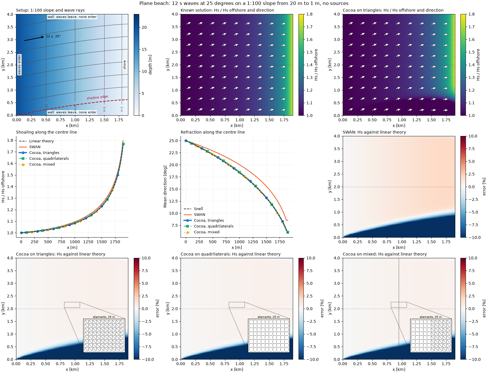
Fig. 49 12 s waves at 25 degrees shoaling and refracting up a 1:100 slope from 20 m to 1 m, with no sources.
A 1.9 by 4 km domain at 25 m spacing, 20 m deep at the western boundary and shoaling at 1:100 to 1 m at the shore. A single frequency and direction bin enters: 12 s at 25 degrees to the shore normal.
With no sources the energy flux \(E c_g \cos\theta\) is conserved and the direction follows Snell’s law. Cocoa’s Hs is within 0.5 % of linear theory along the center line and its direction within 0.23 degrees of Snell. SWAN’s Hs is within 2 %, but its waves refract less: 8.5 degrees at the shore against Snell’s 6.0.
Surf Zone
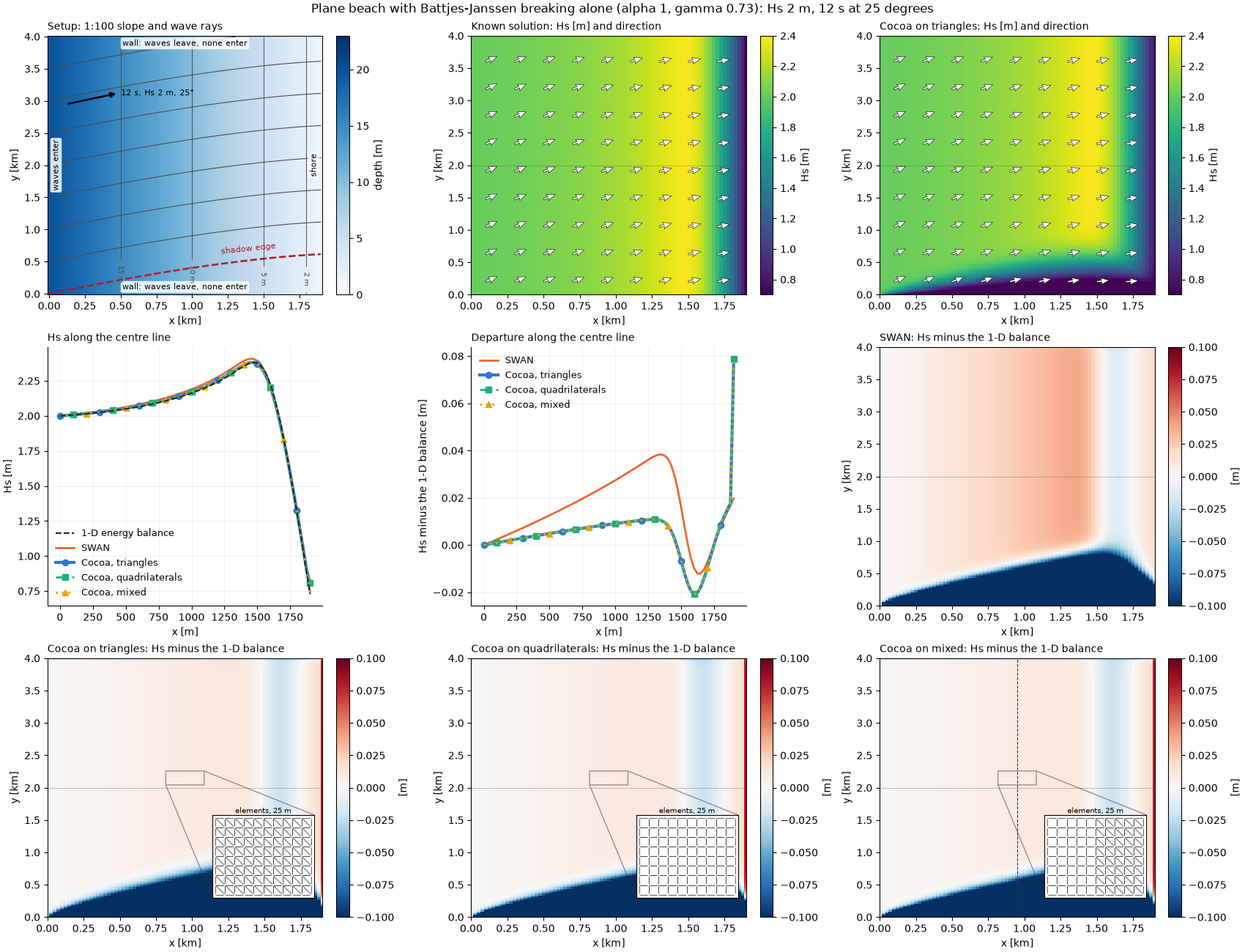
Fig. 50 The same beach with Battjes-Janssen breaking alone (\(\alpha = 1\), \(\gamma = 0.73\)), 2 m incident.
The beach above, with the incident waves raised to 2 m and depth-induced breaking as the only source; the waves break in the last few hundred meters.
The reference is the 1-D energy balance
with \(D_{br}\) from (57), integrated with RK4 from the same breaking and moment code. Hs rises to 2.38 m at 1475 m and then breaks. Cocoa follows the balance to 1.0 % of the incident Hs, identically on the three meshes. At the shore node the gap is 3.9 %, because that node’s control volume is half a cell and its source sits half a spacing from the reference’s point. SWAN departs by up to 3.8 cm, 1.9 %, as it shoals ahead of the balance.
Opposing Current
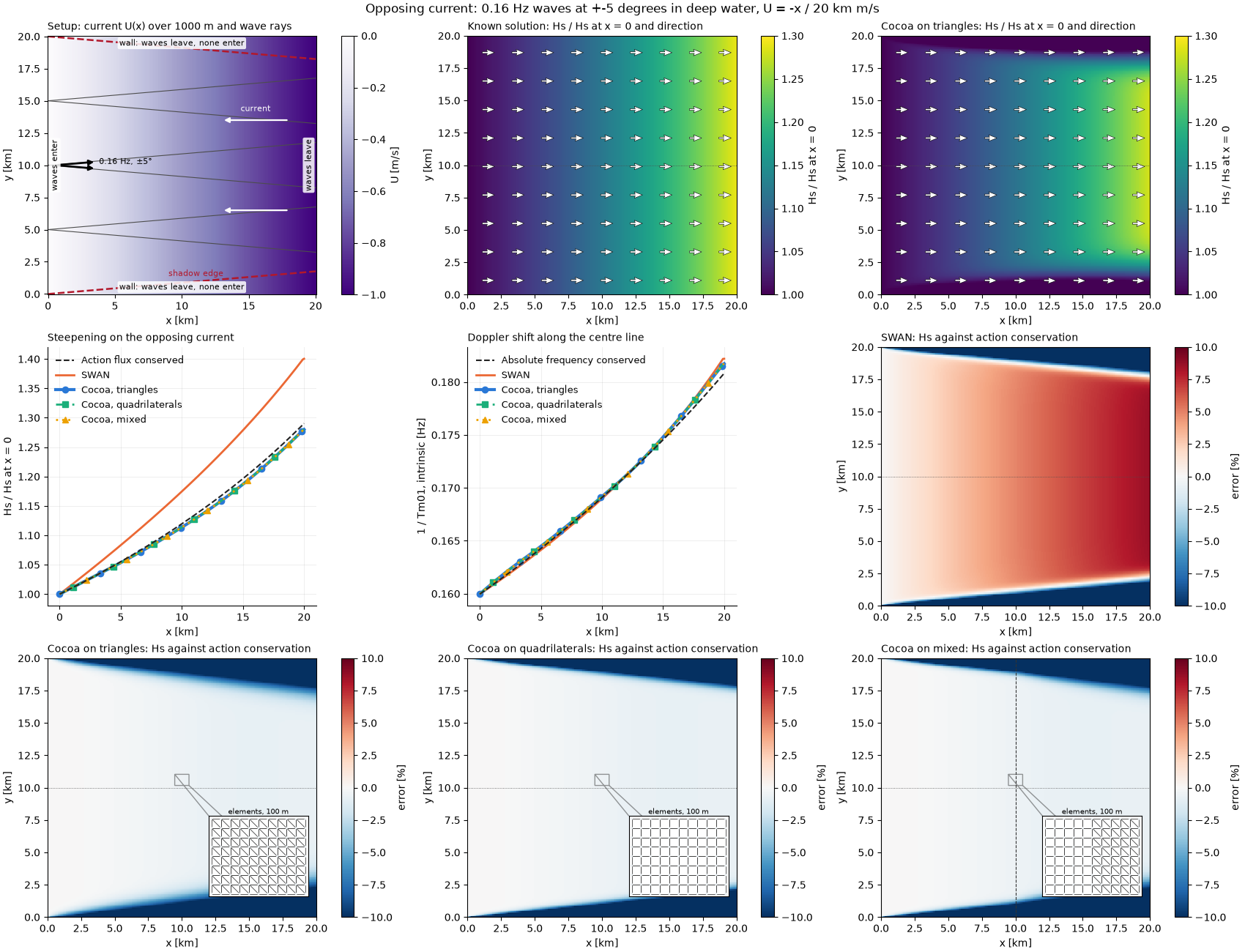
Fig. 51 0.16 Hz waves at \(\pm 5\) degrees in 1000 m of water against a current that grows linearly to 1 m/s over 20 km.
A 20 by 20 km domain at 100 m spacing, 1000 m deep, so depth plays no part. The current flows west, against the waves, growing linearly from zero at the western boundary to 1 m/s at the eastern. The waves enter at 0.16 Hz in the two bins at \(\pm 5\) degrees and steepen as the current slows them.
Along the current the action flux \((c_g\cos\theta + U) N\) and the absolute frequency \(\sigma + kU\cos\theta\) are conserved, which fixes Hs and the intrinsic frequency (dashed). Cocoa’s Hs stays within 0.8 % of that answer; SWAN’s is 8.5 % high at 20 km. The energy-weighted mean intrinsic frequency, \(1/T_{m01}\), is within 0.54 % of exact for Cocoa and 0.8 % for SWAN. The residue is the limiter’s: the incident spectrum is a single bin, a peak, where the correction (51) falls back to first order.
This case is what exposed the frequency-shift error. With upwinding alone, Cocoa’s mean frequency reached 0.190 Hz at 20 km (+5.1 %), and the error halved with each halving of the bin width (+2.3, +1.1, +0.5 % at 5, 2.5 and 1.25 % bins), the signature of first-order diffusion, not of a wrong \(c_\sigma\).
Fetch Growth
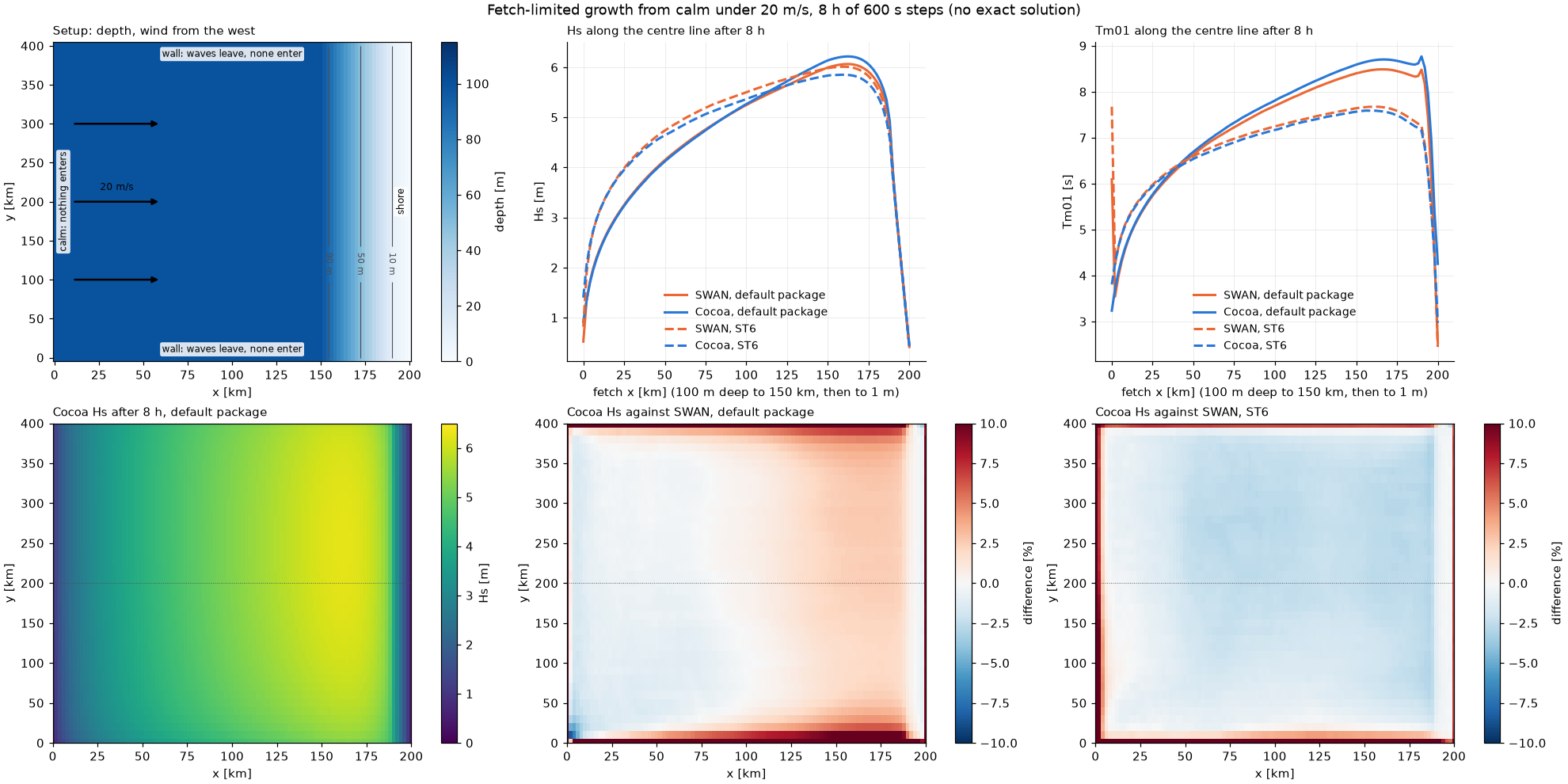
Fig. 52 Growth from calm under 20 m/s along a 200 km fetch, 100 m deep to 150 km and then shoaling to 1 m, after 8 h of 600 s steps.
A 200 by 400 km domain at 2 by 10 km spacing, 100 m deep for 150 km, then shoaling to 10 m at 190 km and 1 m at the shore. The sea starts calm, nothing enters through any boundary, and a uniform 20 m/s wind from the west grows the waves for 8 h. Wind growth has no exact solution, so this problem is Cocoa against SWAN. The top row shows the setup and the two packages along the center line; the bottom row maps Cocoa’s Hs and its difference from SWAN. The boundary nodes differ most, because Cocoa’s boundary dual cells are halves and SWAN’s boundary points are one-sided.
After 8 h Hs and Tm01 along the fetch are within 2.5 % and 2.7 % of SWAN’s with the default package, and within 2.7 % and 1.4 % with ST6. From calm the time step matters. At 1 h SWAN’s own 600 s step runs 16 % higher in Hs than its converged 60 s step. Cocoa’s quadruplets are formed once per step from \(N^n\), so they shift a young sea toward lower frequencies later. With ST6 at 600 s steps, Cocoa’s sea is 34-37 % lower than SWAN’s after 1 h, where SWAN’s first steps stop unconverged at their iteration cap. With both codes at 120 s steps the gap is 20 %.
Decay and Coupled Hurricanes
Decay. When the fetch’s wind drops to 5 m/s, ST6’s Hs stays within 1.4 % of SWAN’s for 12 h and its Tm01 within 2.8 %, with both codes at 120 s steps. At 600 s both carry several percent of step error in that decay.
Coupled hurricanes. Against ADCIRC+SWAN on the Katrina (WNAT) and Irene meshes, Hs is within 4.6 and 9.2 cm rms and Tm01 within 0.34 and 0.36 s rms where both models have waves (default package; ST6 on Katrina: 6.5 cm and 0.37 s).
Where the Ideas Came From
Component |
Origin |
Notes |
|---|---|---|
Action balance, spectral speeds, great-circle turning |
SWAN [Booij1999]; WAVEWATCH III |
The standard formulation; |
Source packages (default and ST6), limiter, stop rule |
SWAN [Booij1999] [Ris1997]; ST6 via WAVEWATCH III [Zieger2015] |
Reproduced formula for formula, and the bugs found in SWAN’s ST6 stress sum corrected. |
Coupling schedule, radiation stress, wind and roughness handed over |
ADCIRC+SWAN [Dietrich2011] |
Chosen so a run can be compared with SWAN+ADCIRC directly. |
Implicit unstructured transport with ordered iteration |
WAVEWATCH III and WWM [Roland2012] [Abdolali2020]; SWAN’s vertex sweeps [Zijlema2010] |
The finding that the order, not the implicitness, keeps iteration counts low at coastal Courant numbers is from Cocoa’s own analysis. |
Median-dual finite volumes on triangles and quadrilaterals |
Cocoa |
Chosen over the N-scheme to cover quadrilaterals; M-matrix property shown for the mixed mesh. |
Per-direction dependency order, blocks, block Jacobi on the GPU |
Cocoa, after the discrete-ordinates sweeps of neutron transport [Koch1992] |
Exact solve within a block, deterministic across team schedules. |
Unsplit backward Euler with sources inside the outer iteration |
SWAN’s practice, re-derived |
A split (transport, then sources) step’s steady state depends on the time step; iterating the unsplit system does not. |
Frequency-shift flux: upwind in the matrix plus a deferred, limited second-order correction in \(\ln\sigma\) |
Cocoa, after MUSCL with van Leer’s MC limiter [vanLeer1977]; SWAN blends central and upwind instead |
Keeps the matrix an M-matrix; found necessary by the opposing-current test. |
Relaxed sink rates, the Komen growth cap, ST6 whitecapping relaxation |
Cocoa |
Measured necessary for convergence of this iteration. |
Single-precision spectra, host placement of the starting spectrum |
Cocoa |
Fits the full CPRA Katrina mesh (1.57M nodes, 36 x 41) on a 16 GB GPU. |
References
Booij, N., Ris, R. C., and Holthuijsen, L. H. (1999). A third-generation wave model for coastal regions: 1. Model description and validation. Journal of Geophysical Research, 104(C4), 7649-7666.
Zijlema, M. (2010). Computation of wind-wave spectra in coastal waters with SWAN on unstructured grids. Coastal Engineering, 57(3), 267-277.
Ris, R. C. (1997). Spectral Modelling of Wind Waves in Coastal Areas. PhD thesis, Delft University of Technology.
Dietrich, J. C., et al. (2012). Performance of the unstructured-mesh, SWAN+ADCIRC model in computing hurricane waves and surge. Journal of Scientific Computing, 52(2), 468-497.
Day, C., and Dietrich, J. C. (2021). SWAN ST6 physics. Coastal and Computational Hydraulics Team, North Carolina State University. https://ccht.ccee.ncsu.edu/swan-st6-physics/
Komen, G. J., Hasselmann, S., and Hasselmann, K. (1984). On the existence of a fully developed wind-sea spectrum. Journal of Physical Oceanography, 14, 1271-1285.
Cavaleri, L., and Malanotte-Rizzoli, P. (1981). Wind wave prediction in shallow water: theory and applications. Journal of Geophysical Research, 86(C11), 10961-10973.
Rogers, W. E., Hwang, P. A., and Wang, D. W. (2003). Investigation of wave growth and decay in the SWAN model: three regional-scale applications. Journal of Physical Oceanography, 33, 366-389.
The WAMDI Group (1988). The WAM model: a third generation ocean wave prediction model. Journal of Physical Oceanography, 18, 1775-1810.
Hasselmann, S., Hasselmann, K., Allender, J. H., and Barnett, T. P. (1985). Computations and parameterizations of the nonlinear energy transfer in a gravity-wave spectrum. Part II: Parameterizations of the nonlinear energy transfer for application in wave models. Journal of Physical Oceanography, 15, 1378-1391.
Battjes, J. A., and Janssen, J. P. F. M. (1978). Energy loss and set-up due to breaking of random waves. Proceedings of the 16th International Conference on Coastal Engineering, 569-587.
Madsen, O. S., Poon, Y.-K., and Graber, H. C. (1988). Spectral wave attenuation by bottom friction: theory. Proceedings of the 21st International Conference on Coastal Engineering, 492-504.
Rogers, W. E., Babanin, A. V., and Wang, D. W. (2012). Observation-consistent input and whitecapping dissipation in a model for wind-generated surface waves: description and simple calculations. Journal of Atmospheric and Oceanic Technology, 29, 1329-1346.
Zieger, S., Babanin, A. V., Rogers, W. E., and Young, I. R. (2015). Observation-based source terms in the third-generation wave model WAVEWATCH. Ocean Modelling, 96, 2-25.
Donelan, M. A., Babanin, A. V., Young, I. R., and Banner, M. L. (2006). Wave-follower field measurements of the wind-input spectral function. Part II: Parameterization of the wind input. Journal of Physical Oceanography, 36, 1672-1689.
Tsagareli, K. N., Babanin, A. V., Walker, D. J., and Young, I. R. (2010). Numerical investigation of spectral evolution of wind waves. Part I: Wind-input source function. Journal of Physical Oceanography, 40, 656-666.
Ardhuin, F., et al. (2010). Semiempirical dissipation source functions for ocean waves. Part I: Definition, calibration, and validation. Journal of Physical Oceanography, 40, 1917-1941.
Hwang, P. A. (2011). A note on the ocean surface roughness spectrum. Journal of Atmospheric and Oceanic Technology, 28, 436-443.
Roland, A., et al. (2012). A fully coupled 3D wave-current interaction model on unstructured grids. Journal of Geophysical Research: Oceans, 117, C00J33.
Abdolali, A., et al. (2020). Large-scale hurricane modeling using domain decomposition parallelization and implicit scheme implemented in WAVEWATCH III wave model. Coastal Engineering, 157, 103656.
Koch, K. R., Baker, R. S., and Alcouffe, R. E. (1992). Solution of the first-order form of the 3-D discrete ordinates equation on a massively parallel processor. Transactions of the American Nuclear Society, 65, 198-199.