Test Cases

The test cases below exercise different features. Each is a verification benchmark and a worked example, with a mesh, a configuration file, and a plotting script that generates a summary figure.

The runnable cases live in their own repository, cocoa-examples, which carries additional cases beyond those described here along with configurations for checkpoint/restart, the implicit solver, and output control:

git clone https://github.com/cocoaorg/cocoa-examples
cd cocoa-examples/flow_channel
cocoa -i cocoa_config.yaml

The descriptions below give the expected behavior and verification figures; see the repository for how to run each case.

The cases from the Ideal Channel (Quadrilateral Validation) section on keep their mesh and configuration under test/data/ in this repository. Run one from its directory with the configuration named in its section:

cd test/data/internal_weir
cocoa -i cocoa_config_integration_test.yaml

The configurations shown leave physics.wetting_velocity at its default, linear. The configurations under test/data/ pin wetting_velocity: inertial (see Integration Test Fixtures).

Channel with Flow

A simple rectangular channel with a specified-flow (type 22) boundary on the upstream (left) end and an open tidal boundary on the downstream (right) end. The top and bottom are land boundaries.

Mesh: 100 x 25 node grid, 10 m uniform depth, ~50 km long channel oriented east-west near the equator.

Forcing: 10,000 m³/s steady inflow on the upstream boundary. The tidal boundary has zero amplitude (still water at the outlet). A 2-day hyperbolic tangent ramp is applied to the flow.

Physics: Manning’s n = 0.025, \(\tau_0\) = 0.005, explicit (lumped) GWCE solver with \(\Delta t\) = 2 s, 3-day simulation.

Expected behavior: Water level rises smoothly during the ramp period and reaches a steady gradient by day 2. The upstream end shows the highest elevation (~0.012 m) with a monotonic decrease toward the downstream open boundary. Velocity is approximately uniform across the channel width.

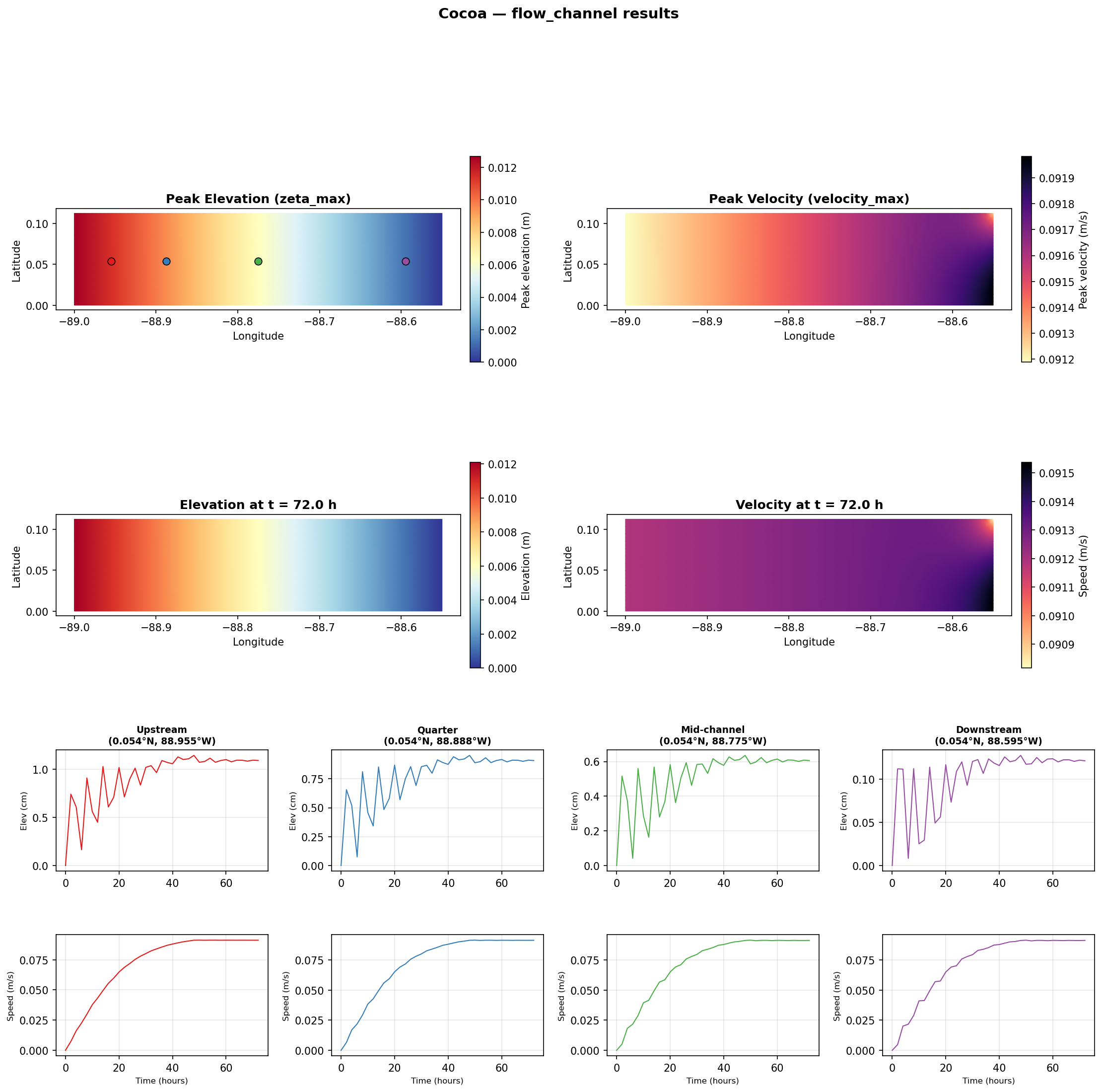
Flow channel (type 22) results showing elevation and velocity maps with probe time series — Fig. 15 Flow channel results. Top row: peak elevation and velocity maps. Middle row: final timestep snapshots. Bottom row: elevation (top) and velocity (bottom) time series at four probe locations along the channel centerline.

Configuration:

output:
  global:
    step_interval: 2h

diagnostics:
  screen_interval: 2h

mesh:
  filename: "flow_channel.nc"
  projection:
    type: "EquidistantCylindrical"
    center: [-89.0, 29.0]

simulation:
  start_time: 2026-01-01
  end_time: 2026-01-04
  time_step: 2s

physics:
  manning_n: 0.025
  cf_lower_limit: 0.0025
  tau0: 0.005

forcing:
  ramp:
    enabled: true
    duration: 2d

  tide:
    potential:
      enabled: false
    boundary:
      enabled: true
      constituents:
        - name: M2
          frequency: 1.4051890280e-04
          nodal_factor: 1.0
          equilibrium_arg: 0.0
          boundary_values:    # 26 open boundary nodes, all zero amplitude
            - { amplitude: 0.0, phase: 0.0 }
            # ... (repeated for all 26 nodes)

  flow_boundary:
    enabled: true
    ramp:
      enabled: true
      duration: 2d
    segments:
      - segment_index: 0
        time_series_file: "flow_segment0.yaml"

initial_conditions:
  water_level: 0.0

The flow time series file (flow_segment0.yaml) prescribes a constant 10,000 m³/s inflow:

time_series:
  - { datetime: "2026-01-01 00:00:00", flow: 10000.0 }
  - { datetime: "2026-02-01 00:00:00", flow: 10000.0 }

The tidal boundary is configured with zero amplitude at all nodes, which amounts to a still-water Dirichlet condition at the downstream open boundary; the tidal forcing section must still be present.

Location: flow_channel/ in the cocoa-examples repository

Channel with Sommerfeld Radiation Boundary and Specified Flow

The same rectangular channel as the type 22 case, but the upstream boundary uses type 32 (specified flow + Sommerfeld radiation) instead of type 22. An M2 tidal signal with 0.005 m amplitude is applied at the downstream open boundary.

Mesh: Identical grid geometry to the flow channel case, but with boundary code 32 on the upstream segment.

Forcing: 10,000 m³/s steady inflow with a prescribed elevation of 0.012 m on the upstream boundary. The downstream boundary has an M2 tidal signal (0.005 m amplitude). Both tidal and flow ramps are 2 days.

Physics: Same as the flow channel case.

Expected behavior: The flow-driven stage ramps up similarly to the type 22 case, but with a superimposed tidal oscillation visible at all probe locations. The radiation term in the \(Q_{\text{force}}\) formulation (see flow boundaries in the GWCE) allows the tidal signal arriving at the upstream boundary to pass through rather than fully reflecting. The upstream probes show the tidal oscillation superimposed on the steady-state flow elevation.

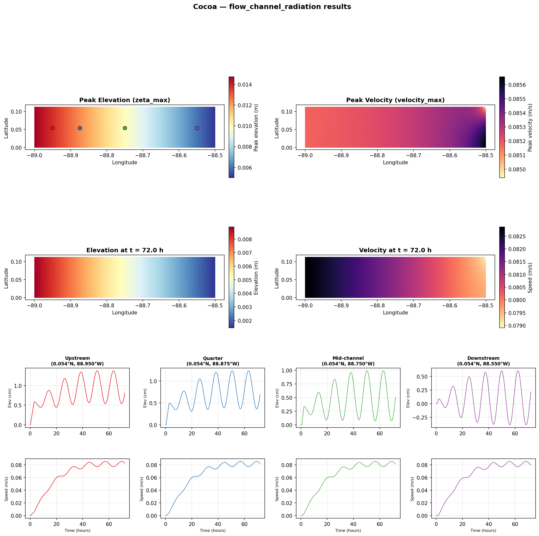
Flow channel with radiation (type 32) results showing tidal oscillation superimposed on flow — Fig. 16 Flow channel with radiation results. The tidal signal from the downstream boundary propagates through the channel and is visible at all probe locations. The upstream probes show tidal oscillation superimposed on the flow-driven stage.

Configuration:

output:
  global:
    step_interval: 60

diagnostics:
  screen_interval: 3600

mesh:
  filename: "flow_channel_radiation.nc"
  projection:
    type: "EquidistantCylindrical"
    center: [-89.0, 0.0]

simulation:
  start_time: 2026-01-01
  end_time: 2026-01-04
  time_step: 2s

physics:
  manning_n: 0.025
  cf_lower_limit: 0.0025
  tau0: 0.005

numeric:
  solver: explicit
  gwce_coefficients: [0.0, 1.0, 0.0]

forcing:
  ramp:
    enabled: true
    duration: 2d

  tide:
    potential:
      enabled: false
    boundary:
      enabled: true
      constituents:
        - name: M2
          frequency: 1.4051890280e-04
          nodal_factor: 1.0
          equilibrium_arg: 0.0
          boundary_values:    # 26 open boundary nodes, uniform 0.005 m
            - { amplitude: 0.005, phase: 0.0 }
            # ... (repeated for all 26 nodes)

  flow_boundary:
    enabled: true
    ramp:
      enabled: true
      duration: 2d
    segments:
      - segment_index: 0
        time_series_file: "flow_segment0.yaml"

initial_conditions:
  water_level: 0.0

The flow time series file for this case includes an elevation field, which is required for the radiation term on type 32 boundaries:

time_series:
  - { datetime: "2026-01-01 00:00:00", flow: 10000.0, elevation: 0.012 }
  - { datetime: "2026-02-01 00:00:00", flow: 10000.0, elevation: 0.012 }

Location: flow_channel_radiation/ in the cocoa-examples repository

Western North Atlantic (WNAT)

A coarse Western North Atlantic domain with tidal and meteorological forcing. This test exercises the full simulation pipeline including tidal boundary conditions, tide potential, meteorological forcing, and wind stress.

Mesh: Coarse unstructured triangular mesh covering the Western North Atlantic, Gulf of Mexico, and Caribbean Sea.

Forcing: M2 tidal constituent on the open ocean boundary with spatially varying amplitude and phase. Tide potential forcing is enabled. CF-NetCDF meteorological forcing provides wind and pressure fields. A 1-day ramp is applied.

Physics: Manning’s n = 0.025, \(\tau_0\) = 0.005, explicit solver with \(\Delta t\) = 20 s, 22-day simulation.

Expected behavior: Tidal oscillations dominate at all probe locations. The Gulf of Mexico probe shows ~1 m tidal range. Wind-driven surge is visible as a low-frequency modulation of the tidal signal. Velocity patterns show strong currents through the Florida Straits and along the shelf break.

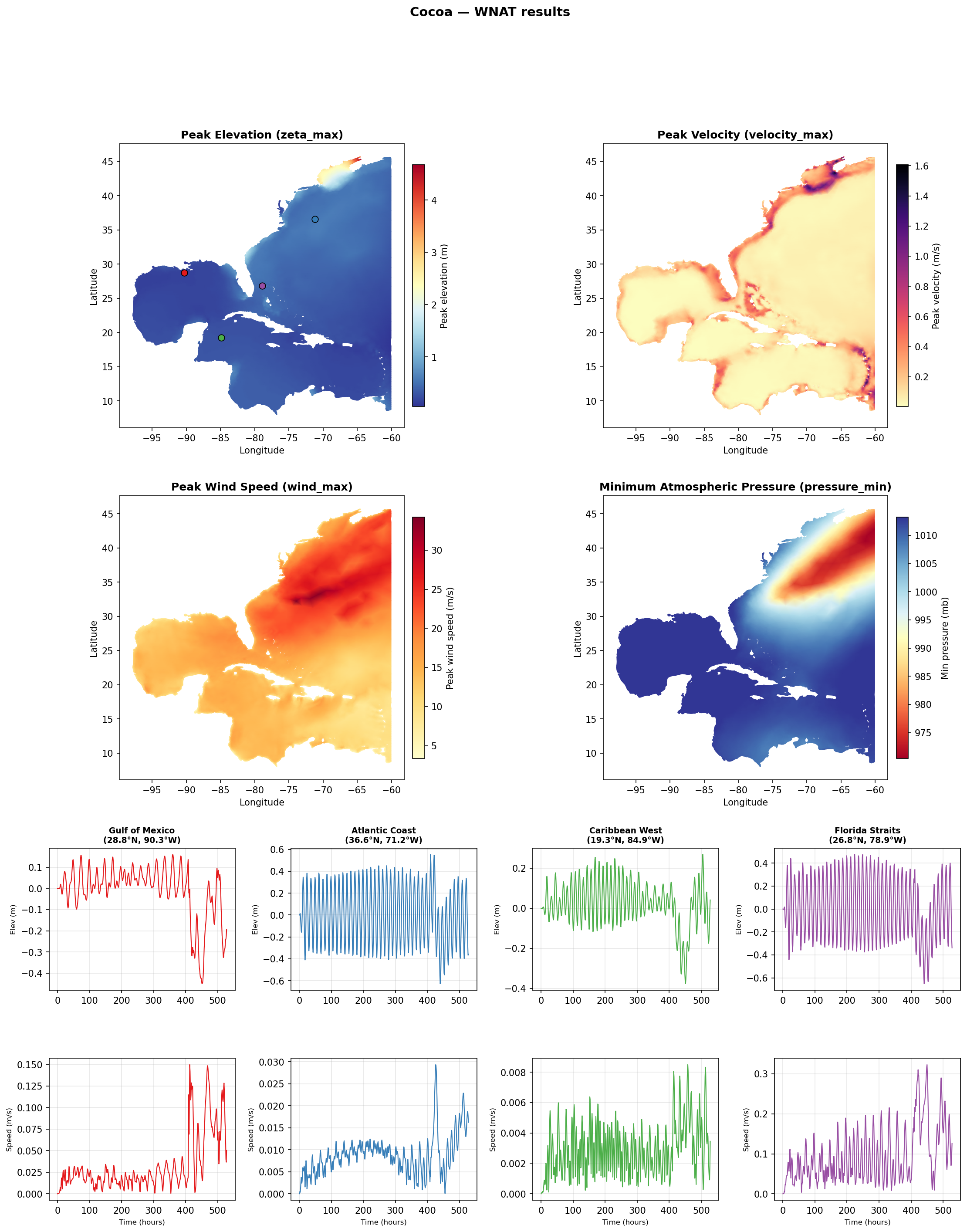
Western North Atlantic results showing tidal and meteorological forcing — Fig. 17 WNAT results. Top row: peak elevation and velocity maps. Middle row: peak wind speed and minimum atmospheric pressure. Bottom row: elevation and velocity time series at four probe locations (Gulf of Mexico, Atlantic Coast, Caribbean West, and Florida Straits).

Configuration (CF-NetCDF meteorological forcing variant):

output:
  global:
    step_interval: 180

diagnostics:
  screen_interval: 180
  log_file: log.json

mesh:
  filename: "wnat.nc"
  projection:
    type: "EquidistantCylindrical"
    center: [-76.572766, 23.241697]

simulation:
  start_time: 2026-01-15
  end_time: 2026-02-06
  time_step: 20s

physics:
  manning_n: 0.025
  cf_lower_limit: 0.0010
  tau0: 0.0050000

numeric:
  solver: explicit
  gwce_coefficients: [0.0, 1.0, 0.0]

forcing:
  meteorological:
    enabled: true
    format: cf_netcdf
    filename: "example_met_data/cf_meteo_example.nc"
  ramp:
    enabled: true
    duration: 1d
  tide:
    potential:
      enabled: true
    boundary:
      enabled: true
      constituents:
        - name: M2
          frequency: 1.405189028e-04
          nodal_factor: 0.964086
          equilibrium_arg: 23.057068
          boundary_values:    # 55 open boundary nodes
            - { amplitude: 5.2403779870e-01, phase: 344.168513 }
            - { amplitude: 5.1732976110e-01, phase: 345.153162 }
            # ... (55 nodes with spatially varying amplitude and phase)

This test case also ships with two alternative meteorological forcing configurations: cocoa_config_owi_ascii.yaml (OWI ASCII format) and cocoa_config_owi_netcdf.yaml (OWI NetCDF format). The only difference between the three is the forcing.meteorological section; all other parameters are identical.

Location: wnat/ in the cocoa-examples repository (configurations and met data), test/data/wnat/ in this repository (integration test data and reference solutions)

Global Ocean

A global ocean mesh test case that exercises coordinate rotation, Mercator projection, and self-attraction and loading (SAL) tide corrections.

Mesh: Global unstructured triangular mesh with coordinate rotation (pole relocated to avoid the North Pole singularity).

Forcing: Astronomical tide potential with SAL correction. No meteorological forcing. A 5-day ramp is applied.

Physics: Manning’s n from mesh (spatially varying), \(\tau_0\) = 0.0022, Smagorinsky lateral viscosity with coefficient 0.2, implicit (consistent) GWCE solver with \(\Delta t\) = 720 s, 31-day simulation.

Expected behavior: Tidal patterns reproduce the expected global amphidromic system. Large tidal ranges appear in shallow shelf regions (Bay of Fundy, Patagonian shelf, European shelf). Deep ocean amplitudes are modest (~0.5 m). The implicit solver allows the large time step.

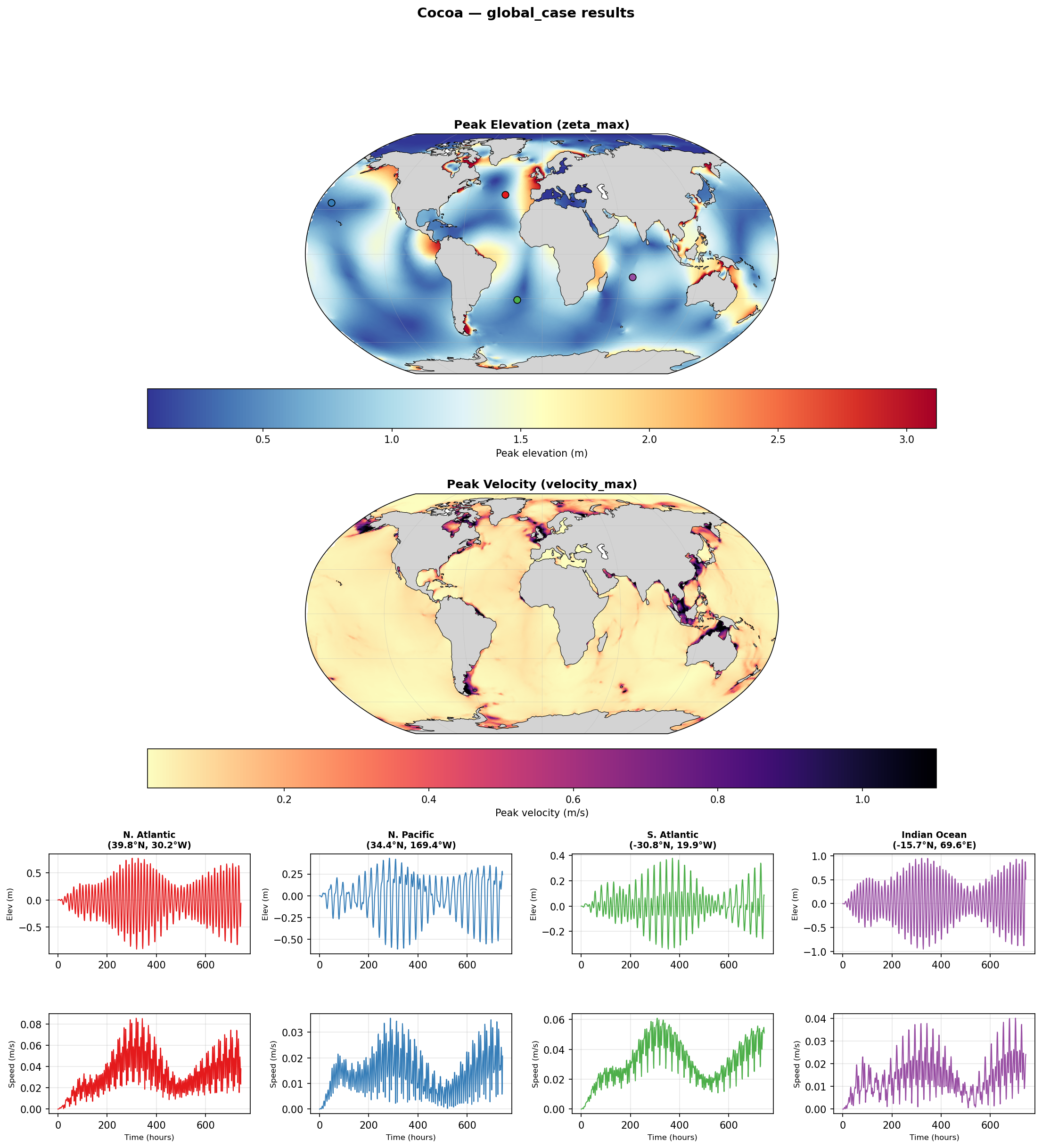
Global ocean results showing tidal amphidromic patterns — Fig. 18 Global ocean results. Top: peak elevation map showing the amphidromic tidal pattern. Middle: peak velocity map. Bottom: elevation and velocity time series at four probe locations (North Atlantic, North Pacific, South Atlantic, Indian Ocean).

The configuration is listed and explained key by key under Complete Example in Global Simulations.

Location: global_case/ in the cocoa-examples repository, test/data/global_case/ in this repository (integration test data and reference solutions)

Ideal Channel (Quadrilateral Validation)

A family of idealized channels used to validate the quadrilateral-element CG solver against triangle-only and hybrid meshes at matched resolution, and both against ADCIRC. Unlike the cases above, these live in this repository as committed fixtures (mesh, configuration and reference solution together under test/data/channel/) instead of in cocoa-examples.

Mesh: Four planforms, each 200 m wide, generated by test/data/channel/make_channel_meshes.py. The straight planform runs 4000 m at constant direction over a flat 10 m bed; meander covers the same 4000 m of arc length over the same bed as a straight 500 m lead-in, a sine-generated reach of three full wavelengths at theta(s) = 30 deg * sin(2*pi*(s - 500 m) / 1000 m), and a straight 500 m lead-out, so both its forcing boundaries sit on straight channel and the centerline is C1 at the two junctions; beach keeps the straight plan geometry and tilts the bed so a tide moves a wet/dry shoreline across it; skewbeach adds a cross-channel tilt to the beach so the shoreline crosses the mesh obliquely. Each planform exists in element-type variants on the same node set (quadrilateral-only, triangle-only, hybrid with quadrilaterals in the middle third, and for the two flat-bed planforms alternating-diagonal triangle and hybrid variants triangle_alt and hybrid_alt) at coarse and fine resolution. The generator self-checks every face for positive (CCW) signed area and quadrilateral convexity before writing. Every mesh also carries explicit mainland natural (ADCIRC type 20) boundary strings along the side walls, and along the tail where the tail is not already an open or flow boundary, so the walls are essential land boundaries at the quad-adjacent nodes instead of being closed only weakly.

Forcing:

Co-oscillating tide (cocoa_config_channel_straight_tide[_implicit].yaml, straight channel only): a single M2 elevation boundary (0.5 m amplitude) at the channel head, closed elsewhere, frictionless (manning_n: 0.0) so the response is the linear standing wave the analytic solution assumes.
Steady uniform flow (cocoa_config_channel_straight_flow.yaml, straight channel only): a specified-flow boundary (ADCIRC type 22, 200 m^3/s prescribed total flow) at the head paired with a fixed z = 0 m boundary at the tail, Manning’s n = 0.025.
Steady flow around the bends (cocoa_config_channel_meander_flow[_implicit].yaml, meander only): the same pair of boundaries at the validation study’s 2000 m^3/s and Manning’s n = 0.025, closed with a constant lateral eddy viscosity of 20 m^2/s (smagorinsky_coefficient: 0.0 with min_viscosity: 20.0, since nu = max(min_viscosity, Cs * Area * abs(S))); why the closure is constant is under Meander.

Physics: Explicit (lumped) and implicit (consistent) GWCE variants for the tide case and for the meander flow case. The straight uniform-flow case is lumped only: at its 4 s step the consistent solver diverges partway through the ramp, and so does ADCIRC’s. The meander runs at a quarter of that step and does not diverge; over 12 h, four times the committed length, its elevation and speed hold at 0.167 m and 1.240 m/s from the third hour on.

Expected behavior: The tide case reaches a bounded, periodic elevation response (well under the 10 m depth) on the hybrid meshes the integration tests run. The two flow cases’ committed runs are short smoke cases, 6 hours on the straight channel and 3 on the meander, where a steady state takes 24.

Hybrid output encoding: a hybrid run’s output NetCDF carries its element connectivity with an nvertex dimension of 4 and a -1 fill value in each triangle row’s unused fourth column. To render a field, cocoa-plot splits each quad along its 0-2 diagonal into two triangles for matplotlib’s Triangulation; the mesh view (-v mesh) draws the actual face edges, so the split never shows as a diagonal.

The segregated strip is also the mesh the quadrilateral partition weight was tuned on; see Mixed-Element Meshes.

Quantitative results. The comparison of every study against its analytic solution and against ADCIRC, at every tier and element variant, with figures, the convergence orders and the validation ctest label that runs them, is Ideal Channel Validation.

Location: test/data/channel/ in this repository (mesh generator, configurations and reference solutions)

Internal Weir

A small tidal domain cut by an internal weir. It exercises the internal weir boundary under explicit tidal forcing, and checkpoint/restart with weirs present. A runnable copy of the case is internal_weir/ in cocoa-examples; the test fixtures and reference below are in this repository. The weir boundary is described under Weir Boundaries.

Mesh: internal_weir.nc: 992 nodes and 1800 triangles spanning 89.0–88.7 deg W and 29.0–29.075 deg N, with depths from 2 to 10 m. One open boundary of 16 nodes and one internal weir boundary (code 24) of 16 node pairs.

Forcing: M2 on the open boundary at 0.5 m amplitude and zero phase on every node, nodal factor 1.0, equilibrium argument 0. No tide potential and no meteorological forcing. A 12-hour ramp is applied.

Physics: Manning’s n = 0.025, \(\tau_0\) = 0.005, explicit solver with \(\Delta t\) = 2 s, 1-day simulation, output every 15 minutes.

Configuration (forcing section of cocoa_config_integration_test.yaml):

forcing:
  ramp:
    enabled: true
    duration: 12h
  tide:
    potential:
      enabled: false
    boundary:
      enabled: true
      constituents:
        - name: M2
          frequency: 1.4051890280e-04
          nodal_factor: 1.0
          equilibrium_arg: 0.0
          boundary_values:    # 16 open boundary nodes
            - { amplitude: 0.5, phase: 0.0 }
            # ... (same value on all 16 nodes)

Location: test/data/internal_weir/ in this repository (mesh, configurations and the reference solution)

GAHM Parametric Vortex (Katrina 2005)

Hurricane Katrina (2005) driven by the GAHM parametric vortex over the WNAT mesh. The fixture exercises vortex-only forcing and a vortex composed with a gridded reader. The vortex model and its configuration keys are described under Parametric Vortex (GAHM).

Mesh: wnat.nc, the WNAT mesh.

Forcing: GAHM vortex from the ATCF track test/data/vortex/katrina_bal122005.dat. No tidal forcing. A 1-hour ramp is applied. The composed configs add a CF-NetCDF reader on example_met_data/cf_meteo_example.nc with a blend_factor of 1.25. That file’s data is in 2026, so the reader never covers the 2005 window and every step takes the vortex-over-background path.

Physics: Manning’s n = 0.025, \(\tau_0\) = 0.005, explicit solver with \(\Delta t\) = 20 s, 6-hour simulation from 2005-08-28 00:00. Output every 2 hours; velocity, pressure and wind output are off, since zeta is the regression quantity.

Configuration (forcing section of cocoa_config_gahm_composed.yaml):

forcing:
  meteorological:
    enabled: true
    format: cf_netcdf
    filename: "example_met_data/cf_meteo_example.nc"
    vortex:
      model: gahm
      tracks:
        - "../vortex/katrina_bal122005.dat"
      blend_factor: 1.25
  ramp:
    enabled: true
    duration: 1h

cocoa_config_gahm_vortex_only.yaml drops format, filename and blend_factor. cocoa_config_gahm_composed_domains.yaml moves the gridded reader into a one-entry domains: list.

Location: test/data/wnat/ (configurations and references) and test/data/vortex/ (track file) in this repository

Sea Ice (WNAT)

Two WNAT runs exercise sea-ice drag attenuation. The ice feature is described under Ice Concentration, and the design of these tests under Testing.

Mesh: wnat.nc, the WNAT mesh.

Forcing: The 1-day WNAT integration setup (cocoa_config_integration_test.yaml): M2 on the open boundary, tide potential with SAL, CF-NetCDF wind and pressure from cf_meteo_example.nc, and a 12-hour ramp. Both runs set meteorological.ice: true.

Zero ice (cocoa_config_zero_ice_test.yaml): the met file is cf_meteo_zero_ice.nc, a copy of cf_meteo_example.nc plus an all-zero siconc variable. It is not committed; generate_cf_meteo_zero_ice.py writes it.
Moving ice: a domains: list composes the wind and pressure source with the ice-only wnat_moving_ice.nc (generate_wnat_moving_ice.py), an ice edge that sweeps south across roughly the northern third of the mesh footprint over 24 hours. ice_drag_law: lupkes.

Physics: Manning’s n = 0.025, \(\tau_0\) = 0.005, explicit solver with \(\Delta t\) = 20 s, 1-day simulation, output every 10 hours.

Configuration (meteorological section of cocoa_config_moving_ice_test.yaml):

forcing:
  meteorological:
    enabled: true
    ice: true
    domains:
      - format: cf_netcdf
        filename: "example_met_data/cf_meteo_example.nc"
      - format: cf_netcdf
        filename: "wnat_moving_ice.nc"
        variables:
          ice: siconc
    ice_drag_law: lupkes

Location: test/data/wnat/ in this repository (configurations, generators and reference)

Baroclinic Forcing (WNAT)

Two WNAT runs exercise baroclinic coupling from a preprocessor-generated nodal forcing file. The coupling is described in Baroclinic Coupling, whose Regression checks section states the invariants these tests pin.

Mesh: wnat.nc for the zero-forcing test. The composed test uses wnat_baroclinic_composed.nc, the WNAT mesh plus a 3-column (Lyard) internal_tide_friction attribute (make_baroclinic_composed_mesh.py), for both its runs.

Forcing: The implicit WNAT setup (cocoa_config_implicit_test.yaml): M2 on the open boundary, tide potential with SAL, no meteorological forcing, and a 12-hour ramp. The baroclinic forcing has its own 12-hour ramp.

Zero forcing: baroclinic_zero_forcing.nc, all zeros (make_baroclinic_zero_forcing.py).
Composed: baroclinic_composed_forcing.nc (make_baroclinic_composed_forcing.py) drives the BPG, free-surface correction, internal-tide drag and dispersion together.

Physics: Manning’s n = 0.025, \(\tau_0\) = 0.005, implicit solver with gwce_coefficients: [0.35, 0.30, 0.35] and \(\Delta t\) = 60 s, 1-day simulation, output every 6 hours.

Configuration (baroclinic keys of cocoa_config_baroclinic_composed_on.yaml):

physics:
  internal_tide_friction: mesh

forcing:
  baroclinic:
    enabled: true
    filename: "baroclinic_composed_forcing.nc"
    internal_tide:
      enabled: true
    dispersion:
      enabled: true
      mode: mld
      deep_water_depth: 1000.0
      mld_coefficients:
        a: 0.01
        b: 0.5

cocoa_config_baroclinic_composed_off.yaml is the same file without these keys. The zero-forcing case runs cocoa_config_baroclinic_zero_forcing.yaml.

Location: test/data/wnat/ in this repository (configurations, generators, forcing files and reference)