Astronomical Tides

Cocoa computes the astronomical tide potential directly, using algorithms from Jean Meeus’s Astronomical Algorithms (2nd ed., 1998) [Meeus1998]: the tide-generating force follows from computed Moon and Sun positions, so no pre-computed harmonic constituents or external ephemeris tables are needed.

Physical Basis

The gravitational tide-generating potential arises from the differential attraction of the Moon and Sun across the Earth. At a point on Earth’s surface, the potential due to a celestial body is:

\[\Phi = \frac{GM}{\Delta} \sum_{n=2}^{\infty} \left(\frac{R_e}{\Delta}\right)^n P_n(\cos\zeta)\]

where:

• \(G\) is the gravitational constant

• \(M\) is the mass of the celestial body (Moon or Sun)

• \(\Delta\) is the distance from Earth’s center to the body

• \(R_e\) is Earth’s radius

• \(P_n\) are Legendre polynomials

• \(\zeta\) is the zenith angle (angle between the observer and the body)

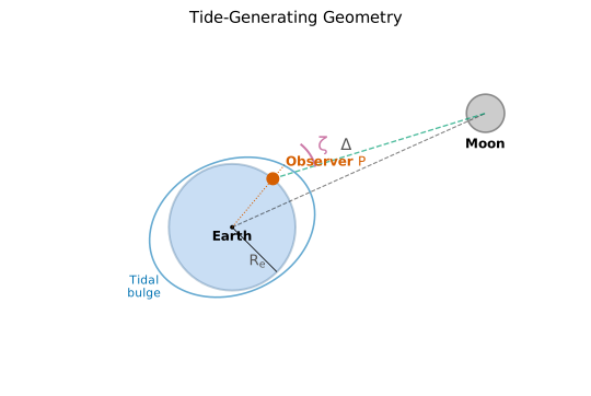
Fig. 42 Tide-generating geometry. The zenith angle \(\zeta\) is measured between the observer’s local vertical and the direction to the Moon (or Sun). The tidal bulge is exaggerated for clarity.

The \(n=1\) term vanishes because it represents uniform translation of the Earth-Moon or Earth-Sun system.

Degree-2 Equilibrium Tide

The dominant contribution comes from the degree-2 (\(n=2\)) term, which produces the familiar equilibrium tide pattern. The second-degree Legendre polynomial is:

\[P_2(\cos\zeta) = \frac{3\cos^2\zeta - 1}{2}\]

This creates a prolate spheroidal water surface with two bulges pointing toward and away from the attracting body.

Higher-Order Terms

Cocoa supports higher-order expansions for improved accuracy, selected by forcing.tide.potential.astronomical.order:

• P2 (order=2): Standard equilibrium tide, fastest computation

• P3 (order=3, the default): Adds the degree-3 term for improved coastal accuracy

• Untruncated (order>=4): Sums the Legendre series through degree 11, adding up to about \(10^{-4}\) m of lunar potential over P3. ADCIRC likewise treats any TIPOrder of 4 or more as the untruncated form.

The degree-3 term uses:

\[P_3(\cos\zeta) = \frac{5\cos^3\zeta - 3\cos\zeta}{2}\]

The untruncated form evaluates the series term by term through the Legendre recurrence \(n P_n = (2n-1)\cos\zeta\, P_{n-1} - (n-1) P_{n-2}\) and stops at degree 11, where the remaining tail is below double-precision roundoff relative to the degree-2 term even at the Moon’s closest perigee. This departs from ADCIRC on purpose. ADCIRC evaluates the equivalent closed form \(1/\sqrt{1 + e^2 - 2e\cos\zeta} - e\cos\zeta - 1\), with \(e = R_e/\Delta\), which builds a quantity of order \(e^2\) out of terms of order one and loses the Sun’s contribution to cancellation. The summed series cancels nothing and is accurate to roundoff for both bodies (untruncated_bracket in forcing/tide/potential/astronomical/AstronomicalTidePotential.cpp).

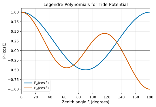
Fig. 43 Legendre polynomials \(P_2(\cos\zeta)\) and \(P_3(\cos\zeta)\) used in the tide-generating potential expansion.

Jean Meeus Algorithms

Cocoa uses algorithms from Meeus’s Astronomical Algorithms to compute celestial body positions analytically with sub-arcminute accuracy. These polynomial and periodic series expressions eliminate the need for external ephemeris tables.

Julian Day and Time

All calculations use Julian Day Number (JD), with time measured in Julian centuries (\(T\)) from the J2000.0 epoch (January 1, 2000, 12:00 TT):

\[T = \frac{\text{JD} - 2451545.0}{36525}\]

Moon Position (Chapter 47)

The Moon’s geocentric position is computed using a 60-term periodic series from Meeus Chapter 47. The algorithm computes:

1. Mean elements: Mean longitude, mean anomaly, mean elongation, and argument of latitude using polynomial expressions in \(T\)

2. Periodic corrections: Additive corrections using sine series for longitude and latitude, cosine series for distance

3. Ecliptic coordinates: Geocentric ecliptic longitude (\(\lambda\)), latitude (\(\beta\)), and distance (\(\Delta\))

The series achieves accuracy of approximately 10 arcseconds in position and 0.2 kilometers in distance over several centuries.

Key orbital elements computed:

Element	Symbol	Description
Mean longitude	\(L'\)	Moon’s mean angular position
Mean anomaly	\(M'\)	Position in elliptical orbit
Mean elongation	\(D\)	Angular distance from Sun
Argument of latitude	\(F\)	Position relative to ascending node

Sun Position (Chapter 25)

The Sun’s apparent geocentric position uses the simplified algorithm from Meeus Chapter 25:

1. Compute the geometric mean longitude and mean anomaly of the Sun

2. Apply the equation of center (correction for elliptical orbit)

3. Calculate apparent longitude including aberration and nutation

The Sun’s distance is computed as:

\[R = \frac{1.000001018 \times (1 - e^2)}{1 + e\cos\nu}\]

where \(e\) is Earth’s orbital eccentricity and \(\nu\) is the true anomaly.

Sidereal Time (Chapter 12)

Greenwich Mean Sidereal Time (GMST) relates Earth’s rotation to the celestial reference frame:

\[\theta_0 = 280.46061837 + 360.98564736629(JD - 2451545.0) + 0.000387933T^2 - \frac{T^3}{38710000}\]

Greenwich Apparent Sidereal Time (GAST) includes the nutation correction:

\[\theta = \theta_0 + \Delta\psi \cos\epsilon\]

where \(\Delta\psi\) is the nutation in longitude and \(\epsilon\) is the obliquity of the ecliptic.

Nutation and Obliquity (Chapter 22)

Nutation is the periodic oscillation of Earth’s rotation axis caused primarily by the Moon’s orbital precession. Cocoa computes:

• Nutation in longitude (\(\Delta\psi\)): affects right ascension

• Nutation in obliquity (\(\Delta\epsilon\)): affects declination

The mean obliquity of the ecliptic is:

\[\epsilon_0 = 23\ |deg|\ 26'21.448'' - 46.8150''T - 0.00059''T^2 + 0.001813''T^3\]

True obliquity includes the nutation correction: \(\epsilon = \epsilon_0 + \Delta\epsilon\)

Coordinate Transformations

Ecliptic to Equatorial

Celestial positions are computed in ecliptic coordinates and transformed to equatorial coordinates (right ascension \(\alpha\), declination \(\delta\)):

\[\tan\alpha = \frac{\sin\lambda\cos\epsilon - \tan\beta\sin\epsilon}{\cos\lambda}\]

\[\sin\delta = \sin\beta\cos\epsilon + \cos\beta\sin\epsilon\sin\lambda\]

Hour Angle and Zenith Angle

The local hour angle relates sidereal time to right ascension:

\[H = \theta - \alpha + \phi_{lon}\]

where \(\phi_{lon}\) is the observer’s longitude.

The zenith angle is computed from:

\[\cos\zeta = \sin\phi_{lat}\sin\delta + \cos\phi_{lat}\cos\delta\cos H\]

where \(\phi_{lat}\) is the observer’s latitude.

Earth Elasticity

The solid Earth deforms in response to tidal forces. This is accounted for using Love numbers:

• \(k_2 = 0.302\): Body tide (elastic deformation of Earth)

• \(h_2 = 0.609\): Vertical displacement of Earth’s surface

The ocean tide amplitude is reduced by the Earth elasticity factor:

\[\alpha = 1 + k_2 - h_2 \approx 0.693\]

The \(k_2\) term adds the potential of the deformed solid Earth to the astronomical potential, while the \(h_2\) term removes the rise of the sea floor itself, which carries the water with it and does not change the water column; the net effect is a reduction. The factor is applied to every degree of the expansion.

Implementation Details

The computation is split between host and device:

HOST (once per timestep):

1. Compute Julian Day from simulation DateTime

2. Calculate Moon position using Meeus Chapter 47 series

3. Calculate Sun position using Meeus Chapter 25

4. Compute GMST from Meeus Chapter 12

5. Transform to equatorial coordinates

DEVICE (parallel over wet mesh nodes):

1. Compute local hour angles for Moon and Sun

2. Calculate zenith angles at each node

3. Evaluate Legendre polynomial expansion

4. Apply Earth elasticity factor and ramp

5. Add the self-attraction and loading term, when SAL constituents are configured

The latitude-dependent trigonometric factors (\(\cos\phi\), \(\sin\phi\)) are precomputed and stored on the device to avoid redundant calculations.

References

The ephemeris algorithms follow [Meeus1998]. Classical harmonic developments of the tide-generating potential are given by [Doodson1921] and [CartwrightTayler1971], and the Love-number treatment of the body tide by [Wahr1981].