Parametric Vortex (GAHM)

Cocoa can generate a tropical-cyclone wind and pressure field analytically from a storm track, instead of (or in addition to) reading gridded meteorological data. The parametric model is the Generalized Asymmetric Holland Model (GAHM) [Gao2013], an asymmetric extension of the classic Holland [Holland1980] profile that fits a separate radius-to-maximum-wind and Holland $B$ shape parameter to each storm quadrant and each reported wind-speed isotach. The vortex is evaluated on the device (GPU or CPU) directly at the mesh nodes every time step, so no external wind file is required for a synthetic or best-track storm.

Overview 

The vortex is the innermost meteorological “domain”: at each node it overlays whatever lies beneath it – a gridded background, the ambient constants, or a previously applied storm – inside the storm footprint, fading to the underlying field through a blend ring at the edge (see Blend ring). The resulting 10 m wind and sea-level pressure feed the same wind-stress and pressure-gradient forcing as gridded meteorology, including the ramp and the wind-reduction pipeline documented in Meteorological Forcing.

Theory 

GAHM builds a per-quadrant wind and pressure field from a handful of track scalars by fitting a modified Holland profile that retains the Coriolis term. This section sketches the equations Cocoa evaluates; they live in cocoa_vortex/physics/GahmPhysics.hpp. Full derivations are in [Gao2013]; the underlying analytic wind and pressure profile is the Holland model [Holland1980] and its revision [Holland2010].

Holland profile and its limitation 

The classic Holland [Holland1980] model sets the profile shape from a single parameter

\[B = \frac{\rho_a\, e\, v_\mathrm{max}^2}{\Delta p}, \qquad \Delta p = p_n - p_c,\]

with air density $\rho_a$, Euler’s number $e$, and the pressure deficit $\Delta p$ between the environmental pressure $p_n$ and the central pressure $p_c$. Its wind follows from cyclostrophic balance – pressure gradient against centrifugal force only. Dropping the Coriolis term is accurate near the eyewall of an intense storm but degrades the fit far from the center and for weak or large storms, where rotation is not negligible.

Gradient-wind generalization 

GAHM restores gradient-wind balance (pressure gradient against centrifugal and Coriolis force). The relative importance of rotation is the Rossby number

\[\mathrm{Ro} = \frac{v_\mathrm{max}}{|f|\, R_\mathrm{max}},\]

where $f = 2\Omega\sin(\mathrm{lat})$ is the Coriolis parameter (the scalar physics uses its magnitude $|f|$). A scaling parameter $\varphi$ and a modified shape parameter $B_g$ then generalize Holland’s $B$:

\[\varphi = 1 + \frac{1}{\mathrm{Ro}\,B_g\,(1 + 1/\mathrm{Ro})}, \qquad B_g = B\,\frac{(1 + 1/\mathrm{Ro})\,e^{\varphi - 1}}{\varphi}.\]

The two are coupled ($\varphi$ depends on $B_g$ and vice versa), which is why the fit iterates (below). As $|f| \to 0$ (the equator, or the cyclostrophic limit) $\mathrm{Ro} \to \infty$, $\varphi \to 1$, and $B_g \to B$ – GAHM reduces to Holland exactly; Cocoa returns these limits explicitly near the equator rather than dividing by $|f|$.

The gradient wind actually evaluated, at radius $r$ with $a = R_\mathrm{max}/r$, is

\[V_g(r) = \sqrt{\,v_\mathrm{max}^2\,\bigl(1 + \tfrac{1}{\mathrm{Ro}}\bigr)\, e^{\,\varphi\,(1 - a^{B_g})}\,a^{B_g} + \Bigl(\tfrac{r|f|}{2}\Bigr)^{2}} \;-\; \frac{r|f|}{2},\]

and the surface pressure is

\[p(r) = p_c + (p_n - p_c)\,e^{-\varphi\,(R_\mathrm{max}/r)^{B_g}}.\]

$V_g$ is the boundary-layer wind; the 10 m wind and the final wind vector (frictional inflow turning, translation, and a fixed frame rotation) are assembled from it (see Ten-minute wind and Translation asymmetry).

Per-quadrant isotach fit 

A track snapshot reports, per quadrant, the radius at which the wind falls to each standard isotach (34/50/64 kt). GAHM treats every (quadrant, isotach) pair independently: $(R_\mathrm{max}, B_g, \varphi)$ are chosen so the gradient wind passes through the reported isotach speed $v_i$ at the reported isotach radius $r_i$,

\[V_g(r_i;\, R_\mathrm{max}, B_g, \varphi) = v_i.\]

Cocoa solves this once per snapshot at startup: an inner bracketed Newton iteration on $R_\mathrm{max}$ over $(0, r_i]$ (the wind is monotone in $R_\mathrm{max}$ there, so a step leaving the bracket is halved toward the bound), wrapped in an outer fixed-point iteration that updates $B_g$ – and through it $\varphi$ – until it stops changing. Because the profile is constructed to pass through each isotach, the wind it produces recovers the reported isotach speed at the reported radius by construction. This is exactly the isotach-recovery property the Verification workflow checks; it is a property of the fit, not of any post-hoc calibration.

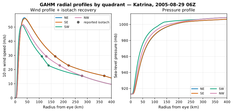
GAHM radial wind and pressure profiles by quadrant for Katrina — Fig. 4 GAHM radial profiles for Hurricane Katrina at its 2005-08-29 06Z near-landfall snapshot, evaluated by Cocoa’s own device-callable physics on a set of radial points. **Left:** the 10 m wind rises to a peak at $R_\mathrm{max}$ (~30 km) and decays outward; the markers are the reported NHC 34/50/64 kt isotachs, and every curve passes exactly through its isotach at $0.89\times$ the reported one-minute speed (the ten-minute equivalent) – the isotach-recovery property, by construction. The four quadrants differ (NE/SE reach 34 kt near 370 km, SW near 278 km): the storm is asymmetric. **Right:** the pressure rises monotonically from the central pressure (~913 mb) toward the environmental pressure, faster in the more compact SW/NW quadrants.

Azimuthal composition 

The four quadrant solutions are stitched into a field continuous in azimuth. At a bearing whose blend angle from one quadrant toward the next is $\theta \in [0, \tfrac{\pi}{2}]$, each solved parameter $X$ is an inverse-square-weighted average of its two bounding-quadrant values:

\[X(\theta) = \frac{w_1 X_1 + w_2 X_2}{w_1 + w_2}, \qquad w_1 = \frac{1}{\theta^2},\quad w_2 = \frac{1}{(\pi/2 - \theta)^2}.\]

The weighting pulls the field to the pure quadrant value on each quadrant centerline ($\theta = 0$ or $\pi/2$); Cocoa returns the exact bounding value within a small tolerance of a centerline to avoid the division-by-zero the raw weights have there. The same weighting sets the azimuthal coverage radius $R_\mathrm{out}(\theta)$ used by the Blend ring.

Translation asymmetry 

A moving storm is asymmetric: its forward motion adds to the wind on one side and subtracts on the other. GAHM removes the storm-translation velocity $\mathbf{U}_t$ from the reported winds before the fit and adds it back after evaluation, so the fit sees a quasi-stationary vortex. The removal is common to both methods below; they differ only in how much motion is removed and how it is re-added.

Removal is a vector quotient – the quadrant isotach speed handed to the solver is the reported speed divided by the magnitude of the quadrant unit vector plus the normalized translation,

\[v_\mathrm{quad} = \frac{v_i} {\bigl\lVert \hat{\mathbf{u}} + \mathbf{U}_t / v_\mathrm{max} \bigr\rVert}.\]

Two re-addition conventions are selectable through env_wind; both follow the GAHM2026 reference [Gao2013] [Luettich2026].

ADCIRC (env_wind: adcirc, the default and Luettich’s recommendation) scales the translation by an empirical function of the eye-to-eye motion between consecutive snapshots,

\[\lVert \mathbf{U}_t \rVert = 1.5\, \left| \frac{\Delta s}{\Delta t} \right|^{0.63} \,(0.51444)^{0.37},\]

where the trailing $(0.51444)^{0.37}$ reconciles GAHM’s knots-based coefficient with the m/s eye motion ($0.51444$ is the knot-to-m/s factor; without it the coefficient silently carries the wrong units). The translation is re-added scaled by the local-to-maximum wind ratio,

\[\mathbf{V}_\mathrm{env} = \mathbf{V} + \mathbf{U}_t\,\frac{\lVert \mathbf{V} \rVert}{v_\mathrm{max}},\]

so the asymmetry is strongest near the radius of maximum winds and fades in the weak outer field.

Lin & Chavez (env_wind: lin_chavez, [LinChavez2012]) removes a smaller fraction of the motion and re-adds it as a constant background vector rather than a profile-scaled one:

\[\lVert \mathbf{U}_t \rVert = 0.6\,\left| \frac{\Delta s}{\Delta t} \right|, \qquad \mathbf{V}_\mathrm{env} = \mathbf{V} + \mathcal{R}_{20^\circ}\,\mathbf{U}_t,\]

where $\mathcal{R}_{20^\circ}$ rotates the translation vector $20^\circ$ from the storm heading (toward the low, i.e. counterclockwise in the Northern Hemisphere and clockwise in the Southern, via $\operatorname{sign}(\text{lat})$). The constant re-add is applied only inside the storm footprint, so the ambient field outside the blend ring is untouched.

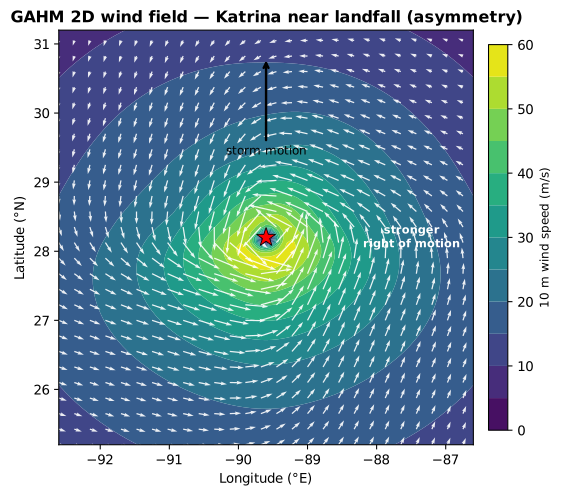
GAHM 2D wind field for Katrina near landfall showing the asymmetry — Fig. 5 The GAHM 2D wind field for the same Katrina snapshot, produced by solving the vortex on a structured longitude/latitude grid and plotting the result. The wind circulates counterclockwise about the eye (a Northern-Hemisphere storm); the arrows are the wind vectors and the fill is wind speed. The field is **asymmetric**: with the storm moving north, the translation adds to the wind on the right of motion (the eastern flank), which – together with the wider reported isotachs there – makes the eastern half stronger and broader than the western half. A Southern-Hemisphere storm mirrors this, circulating clockwise (see Southern Hemisphere).

From theory to code 

The fit – the Newton/fixed-point solve of $(R_\mathrm{max}, B_g, \varphi)$ per quadrant and isotach, plus the translation preparation – runs on the host, once at startup, in cocoa_vortex/solver (GahmSolver and GahmPreprocessor). The closed-form evaluation – gradient wind, pressure, azimuthal blend, and wind-vector assembly – lives in cocoa_vortex/physics/GahmPhysics.hpp as KOKKOS_INLINE_FUNCTION routines, so the host reference evaluator and the device overlay kernel call the same functions and agree to floating-point tolerance (see Solve-once, interpolate-packs).

Configuration 

The vortex is configured under forcing.meteorological.vortex. Meteorological forcing may run with only a vortex, only a gridded reader, or both; enabled: true requires at least one of format/filename or vortex.

Key	Default	Description
`model`	`gahm`	Parametric model. `gahm` is the only accepted value.
`tracks`	(required)	Non-empty list of ATCF track files (best-track, or a preprocessed single-cycle forecast – see Forecast tracks), applied in list order.
`blend_factor`	`1.25`	Outer edge of the blend ring as a multiple of the outermost isotach radius. Must be $\ge 1.0$.
`wind_reduction`	`true`	Apply the land wind-reduction corrections (directional roughness and canopy) to the vortex wind before it is blended. Defaults on: a parametric vortex is a marine 10 m wind that should be reduced to a land surface wind. Set `false` to leave it unreduced (e.g. when composing over a gridded field that already carries the reduction). Only takes effect when the mesh carries the reduction attributes – see Meteorological Forcing.
`pressure_estimate`	`courtney_knaff_2009`	Wind-pressure relationship used to fill a missing central pressure (forecast a-decks omit MSLP). One of `courtney_knaff_2009`, `knaff_zehr_2007`, `dvorak_1984`, `atkinson_holliday_1977`, or `none` (fail loud on a missing pressure). See Estimating a missing central pressure.
`pressure_anchor_hours`	`48`	Bias-offset anchoring window [h] that smooths the hindcast-to-forecast pressure seam in a combined best-track + forecast file. `0` disables anchoring (pure per-snapshot estimate).
`env_wind`	`adcirc`	Storm-motion (environmental wind) re-addition convention: `adcirc` (profile-scaled, the empirical GAHM re-add) or `lin_chavez` (constant background vector rotated $20^\circ$). See Translation asymmetry.
`boundary_layer_factor`	`0.9`	Gradient-wind-to-10 m boundary-layer reduction applied to the top-of- boundary-layer wind. Must lie in $[0.75, 0.9]$; `0.9` is the GAHM default. See Ten-minute wind.
`ramp`	`0` (off)	Duration of the activation/deactivation cross-fade applied as each storm’s own track data window opens or closes (e.g. `6h`), referenced to that track’s first and last snapshot times. Folded into the storm’s spatial blend ring (Blend ring) rather than a separate step. Distinct from the top-level `forcing.ramp` cold-start spinup ramp (see Meteorological Forcing), which fades the whole composed field in once at the start of the run; the equivalent per-source key for a gridded `domains:` entry is documented at Activation Ramp.

Vortex-only 

With no format/filename, the provider runs in vortex-only mode: the vortex is overlaid on the ambient background pressure and zero wind.

forcing:
  meteorological:
    enabled: true
    vortex:
      model: gahm
      tracks:
        - "katrina_bal122005.dat"
      blend_factor: 1.25
  ramp:
    enabled: true
    duration: 1h

Composed with a gridded background 

A gridded reader and a vortex can be combined. Where both are active the vortex rides on the interpolated gridded field; outside the gridded data’s time window the vortex still applies over the ambient background. The provider’s effective data window is the union of the reader window and the vortex track window.

Each gridded domain and each vortex track announces itself in the log when the simulation first enters and leaves its data window, so a run’s log records when each source was actually forcing the solution. A track whose window never overlaps the simulated period produces a warning.

forcing:
  meteorological:
    enabled: true
    format: cf_netcdf
    filename: "background_met.nc"
    vortex:
      model: gahm
      tracks:
        - "storm.dat"
      ramp: 6h                              # fade the storm in/out at its own track window edges
  ramp:
    enabled: true
    duration: 12h

Multiple storms 

Listing more than one track overlays several storms in a single run. Storms are applied in list order, so a later entry wins in an overlap: inside a later storm’s footprint the earlier storm becomes the underlying field that the later storm blends against.

forcing:
  meteorological:
    enabled: true
    vortex:
      model: gahm
      tracks:
        - "storm_a.dat"   # underlying where they overlap
        - "storm_b.dat"   # wins the overlap

The optional ramp key applies per storm: each track fades in and out against its own first and last snapshot times, so two storms whose tracks cover different periods activate and retire independently even though they share the one configured duration.

Blend ring 

Each storm has full weight inside R_out (the outermost, i.e. weakest, reported isotach radius, blended around the azimuth), then ramps linearly to zero weight at blend_factor * R_out and applies nothing beyond. This avoids a hard discontinuity at the storm edge. The blend against the underlying field is a plain linear interpolation of the wind components and pressure, which is correct when the underlying field may point in a different direction from the vortex wind.

When ramp (Configuration) is set, this same per-node ring weight is additionally multiplied by the storm’s own activation/deactivation cross-fade, referenced to the track’s first and last snapshot times, so the whole ring – not only the vortex core – fades in and out smoothly as the track’s window opens and closes.

Physics conventions 

Ten-minute wind 

ATCF best tracks report a one-minute maximum sustained wind. GAHM works in ten-minute winds, so the one-to-ten-minute conversion factor (0.89) is applied early, during track preprocessing, before the Rmax/$B_g$ solve. Reported isotach wind speeds are treated consistently. The peak 10 m wind produced at the radius of maximum winds therefore tracks vmax * 0.89 * (boundary-layer factor) rather than the raw one-minute vmax.

The boundary-layer factor reduces the gradient (top-of-boundary-layer) wind to the 10 m wind. It is configurable through boundary_layer_factor over the physically defensible range $[0.75, 0.9]$; the default 0.9 is the GAHM value. Lower values within the range yield a weaker surface wind for the same gradient wind, and the reported-isotach recovery holds at any setting because the same factor is applied on both the removal and evaluation sides of the fit.

Southern Hemisphere 

Southern-Hemisphere storms (negative latitude, SH basin) are supported: the Coriolis sign flips and the tangential wind sense reverses (clockwise rotation). The wind magnitude differs legitimately from the Northern- Hemisphere mirror because the translation-asymmetry preparation is itself hemisphere-dependent – under env_wind: lin_chavez the $20^\circ$ storm-motion rotation follows $\operatorname{sign}(\text{lat})$, so it turns the opposite way in the two hemispheres.

Solve-once, interpolate-packs 

For each track snapshot Cocoa solves the per-quadrant, per-isotach GAHM parameters once at preprocessing. Between snapshots it linearly interpolates the solved parameters (radius-to-max-wind, $B_g$, the scaling parameter $\varphi$) and the storm scalars (eye position, central pressure, translation), rather than re-solving at every model time step. This is a deliberate, documented deviation from re-solving on every query: at a snapshot time the interpolation weight is 0 or 1, so evaluation reduces exactly to a single snapshot – the state against which the committed regression references are generated, so the deviation does not affect them. In MPI runs every rank preprocesses the (tiny) track identically, with no communication.

Track input (ATCF)

Tracks are comma-delimited ATCF files, one record per line. Cocoa parses the basin, cycle time, forecast hour, eye position, one-minute vmax, central pressure, and the wind-radii (34/50/64 kt) quadrant records. Best-track (b-deck) and forecast (a-deck) files share the same column layout; the differences that matter for Cocoa are called out under Forecast tracks. Key expectations:

The forecast-hour column (tau, field 6) is added to the cycle time in whole hours, and the minutes column (field 4) is added within the hour, so both off-synoptic best-track times and multi-hour forecast lead times land on the correct valid time.
Snapshot times must be strictly increasing; out-of-order lines are rejected (they would silently reverse the translation vector).
Same-time lines are merged (multiple isotach records for one valid time); disagreeing storm scalars at the same time are a hard error.
Short (fewer-than-28-column) lines are skipped with a warning, so wave-radii or other non-standard trailing records do not abort the run.
A snapshot whose GAHM solve fails to converge in a quadrant falls back to a converged neighbor (nearest lower isotach in the same quadrant, else another quadrant of the same isotach), logged as a warning; an unrecoverable snapshot fails loud.

Best-track files 

A best-track (b-deck) file – one storm, technique BEST, tau = 0 on every line, chronological – is the intended, drop-in input. NHC b-decks (e.g. bal122005.dat for Katrina) are used directly, no preprocessing required.

Forecast tracks 

NHC also distributes forecast guidance as ATCF a-deck aid files (e.g. aal092021.dat). These share the b-deck column layout, and the tau column already does the right thing: a single forecast cycle expands to a sequence of snapshots at cycle time + 0, +12, +24 … hours, strictly increasing. A forecast a-deck is not a drop-in file, though – prepare it in three steps.

Reduce to one technique and one cycle. An a-deck interleaves every objective aid (CARQ, AVNO, OFCL …) across every advisory in a single file. Cocoa does not filter on the technique (field 5) or the cycle time, so it would merge them all into one track and abort on the first same-time scalar conflict. Extract the official forecast (OFCL) for one cycle:
```
# Hurricane Ida official forecast issued 2021-08-26 12Z
awk -F, '$5 ~ /OFCL/ && $3 ~ /2021082612/' aal092021.dat > ida_ofcl.dat
```
Central pressure is estimated automatically. NHC forecasts intensity as the maximum wind, not the minimum sea-level pressure, so the MSLP field is 0 on most forecast lines. GAHM needs the pressure deficit $\Delta p = p_n - p_c$ to fit Holland’s $B$. By default Cocoa estimates a missing central pressure from the reported wind using a wind-pressure relationship (see Estimating a missing central pressure), warning for each fill; a reported pressure is never modified. Set vortex.pressure_estimate: none to instead fail loud on a missing pressure.
Blank the technique-number field. On a best track, field 4 carries the observation minutes; on an a-deck it carries the technique sort number (03 for OFCL), and Cocoa reads field 4 as minutes either way – so an unedited OFCL line shifts its valid time by +3 minutes. Blank that field (or accept the fixed, surge-irrelevant three-minute offset). This does not affect the tau column (field 6), which continues to add whole forecast hours.

A best-track file needs none of these steps.

Estimating a missing central pressure 

Theoretical basis. In gradient-wind balance the radial pressure gradient is set against the centrifugal and Coriolis forces, which makes the central pressure deficit a monotonic function of the maximum wind: a stronger wind implies a deeper storm. A wind-pressure relationship (WPR) inverts that link to recover $p_c$ from the reported $v_\mathrm{max}$. The simplest WPRs are single-variable curve fits calibrated to a basin; the modern operational methods add the covariates the balance actually depends on – latitude (through the Coriolis parameter), storm size (a broader wind field integrates to a deeper $p_c$ at the same $v_\mathrm{max}$), and translation speed (a moving storm’s ground-relative peak wind includes its motion, so it is the storm-relative wind that maps to $p_c$).

Cocoa fills a missing central pressure (the 0 MSLP sentinel) from one of the following, selected by vortex.pressure_estimate:

`pressure_estimate`	Reference	Basis
`atkinson_holliday_1977`	[AtkinsonHolliday1977]	Western North Pacific single-curve fit $p_c = 1010 - (v_\mathrm{max}/3.4)^{1/0.644}$ (hPa, m/s).
`dvorak_1984`	[Dvorak1984]	Satellite-intensity single-curve fit $p_c = 1015 - (v_\mathrm{max}/3.92)^{1/0.644}$.
`knaff_zehr_2007`	[KnaffZehr2007]	Reduced single-curve fit $p_c = 1010 - (v_\mathrm{max}/2.3)^{1/0.760}$.
`courtney_knaff_2009` (default)	[CourtneyKnaff2009]	Operational NHC method: a storm-relative maximum wind $V_\mathrm{srm} = v_\mathrm{max} - 1.5\,V_t^{0.63}$, a latitude-piecewise pressure drop, and a size parameter from the 34 kt radius (or climatological when absent). This is how NHC assigns a pressure when only the wind is forecast, so it is the default.

The estimate uses the reported one-minute $v_\mathrm{max}$. Only missing pressures are filled – a reported pressure is never modified – and each fill is logged as a warning naming the storm, time, wind, method, and resulting pressure. pressure_estimate: none disables estimation and restores the fail-loud-on-missing behavior. A missing pressure with no usable wind, or an estimate that yields a non-positive deficit against $p_n$, fails loud.

Combined best-track + forecast files. When observed pressures precede a run of missing (forecast) pressures in one file, a raw WPR estimate at the first forecast time can differ from the last observed value (a WPR is a statistical fit, and a given storm sits off the curve), producing an unphysical jump at the hindcast-to-forecast seam. Cocoa removes that jump by bias-offset anchoring: at the last valid pressure it measures observed - WPR and carries that offset into the following estimates, decaying it linearly to zero over vortex.pressure_anchor_hours (default 48 h; 0 disables anchoring, giving a pure per-snapshot estimate). With no preceding valid pressure – a pure forecast – anchoring is inert and the estimate is the plain WPR.

forcing:
  meteorological:
    vortex:
      model: gahm
      tracks: [storm.dat]
      pressure_estimate: courtney_knaff_2009   # or none / dvorak_1984 / ...
      pressure_anchor_hours: 48                # seam anchoring window; 0 = off

Verification workflow 

utils/plot_gahm_profile.py renders the radial wind and pressure profiles a track produces, per quadrant, with the reported NHC isotach points overlaid. This is the visual acceptance check for a storm: the plotted wind at each reported isotach radius should pass through that isotach’s speed scaled by the 0.89 one-to-ten-minute factor (the isotach-recovery property – GAHM is fit to the ten-minute equivalent of each reported one-minute isotach, so the curve recovers 0.89 x the reported speed at the reported radius, uniformly across quadrants). This holds by construction of the fit, not by calibration – see Per-quadrant isotach fit under Theory. The pressure profile should rise monotonically from the central pressure at the eye toward the environmental pressure, and the peak wind should sit at the radius of maximum winds.